Week 10 - Simulating Combustion of Natural Gas.
Aim: To perform the combustion simulation of natural gas and Generate a plot for CO2, H2O, CH4, N2, O2, NOx emissions & Soot formation.
Theory:
About the Natural Gas:
Natural gas (also called fossil gas or simply gas) is a naturally occurring mixture of gaseous hydrocarbons consisting primarily of methane in addition to various smaller amounts of other higher alkanes. Usually low levels of trace gases like carbon dioxide, nitrogen, hydrogen sulfide, and helium are also present. Natural gas is colorless and odorless, so odorizers such as mercaptan, which smells like sulfur or rotten eggs, are commonly added to natural gas supplies for safety so that leaks can be readily detected.
Natural gas is a fossil fuel and non-renewable resource that is formed when layers of organic matter (primarily marine microorganisms) decompose under anaerobic conditions and are subjected to intense heat and pressure underground over millions of years.The energy that the decayed organisms originally obtained from the sun via photosynthesis is stored as chemical energy within the molecules of methane and other hydrocarbons.
Natural gas can be burned for heating, cooking, and electricity generation. It is also used as a chemical feedstock in the manufacture of plastics and other commercially important organic chemicals and less commonly used as a fuel for vehicles.
Combustion Process:
When natural gas burns, a high-temperature blue flame is produced and complete combustion takes place producing only water vapor and carbon dioxide. It has a heating value of about 1000 BTUs per cubic foot. However, when it burns improperly, it can produce carbon monoxide – a deadly, poisonous gas.
Theory
Combustion is complex reaction which involves chemical kinetics.
CH4+2O2→CO2+2H2O .
But the presence of several inbuilt models like eddy dissipation, finite rate chemistry, finite rate eddy dissipation model etc. to find source of combustion in no time and as a result it allows us to plot mass fraction plots, contours of temperature and velocity, which is very helpful to visualize flame propagation, hot spot etc.
Flames are of two types:
Premixed flame and
Non premixed flame or diffused flame
In our model we assume that the combustion starts due to turbulence and takes place place without any external ignition source.
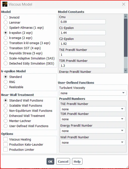
Eddy dissipation model - The eddy dissipation model is based on the concept that chemical reaction is fast relative to the transport processes in the flow. When reactants mix at the molecular level, they instantaneously form products. The model assumes that the reaction rate may be related directly to the time required to mix reactants at the molecular level.
The eddy dissipation model was developed for use in a wide range of turbulent reacting flows covering premixed and diffusion flames. Because of its simplicity and robust performance in predicting turbulent reacting flows, this model has been widely applied in the prediction of industrial flames.
The finite chemistry model –
The finite-rate chemistry model allows the computation of reaction rates described by the molecular interaction between the components in the fluid. It can be combined with the eddy dissipation model for flames where chemical reaction rates might be slow compared with the reactant mixing rates. The finite-rate chemistry model is best applied to situations where the chemical time scale is rate-limiting. This model can be used in conjunction with both laminar and turbulent flow.
The flamelet model –
The flamelet model can provide information on minor species and radicals, such as CO and OH, and accounts for turbulent fluctuations in temperature and local extinction at high scalar dissipation rates, for the cost of solving only two transport equations. The model is only applicable for two-feed systems and requires a chemistry library as input. The model can be used only for non-premixed systems.
Burning velocity model and the extended coherent flame model –
The burning velocity model (BVM) and the extended coherent flame model (ECFM) model the propagation of a premixed or partially premixed flame by solving a scalar transport equation for the reaction progress. The BVM uses an algebraic correlation for modelling the turbulent burning velocity. When using the ECFM, the turbulent burning velocity is closed by solving an additional transport equation for the flame surface density.
Geometry Setup
Given Geometry model file
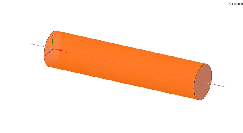
Now we convert the 3d component in to 2d component since the component is symmetric about the x-axis and 2d models allows us for less computational power.
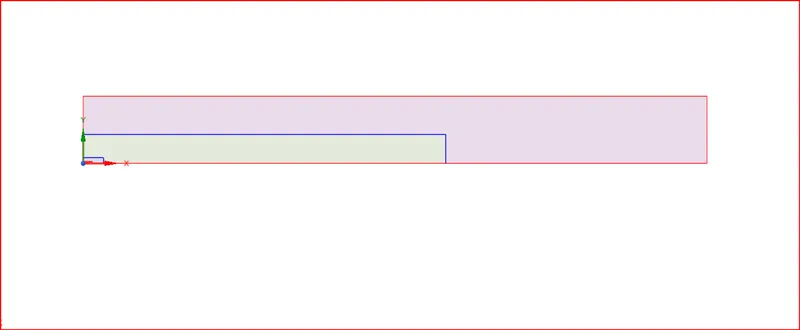
Insert planes at the origin and byusing split body command cut the component along the xy plane and xz plane .
Now select the face and copy it in the new design file to extract the 2d model.
Meshing
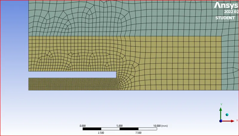
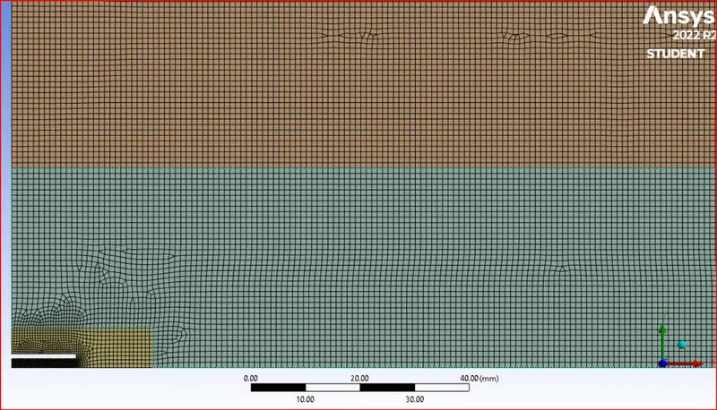
Create the Named selection and generate the mesh
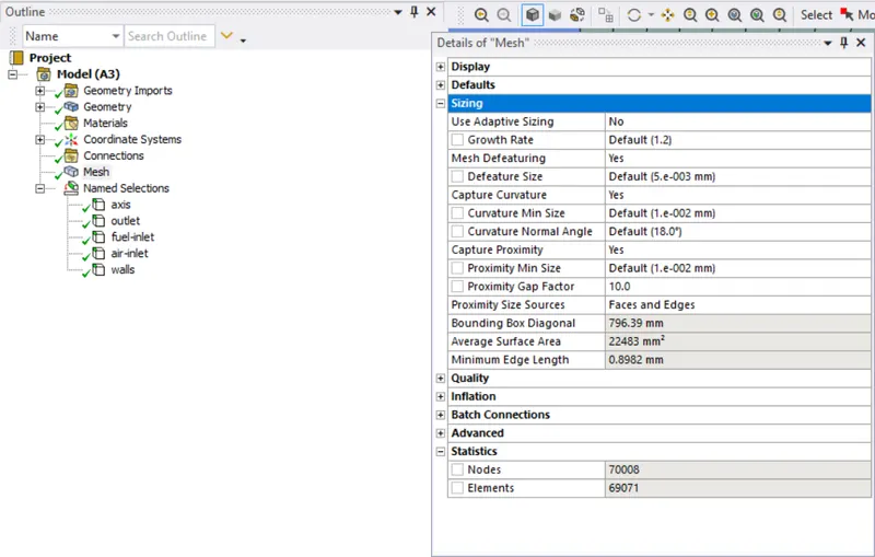
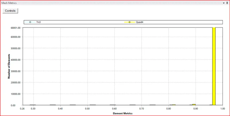
Mesh metrics
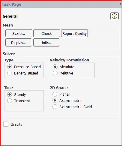
Fluent setup
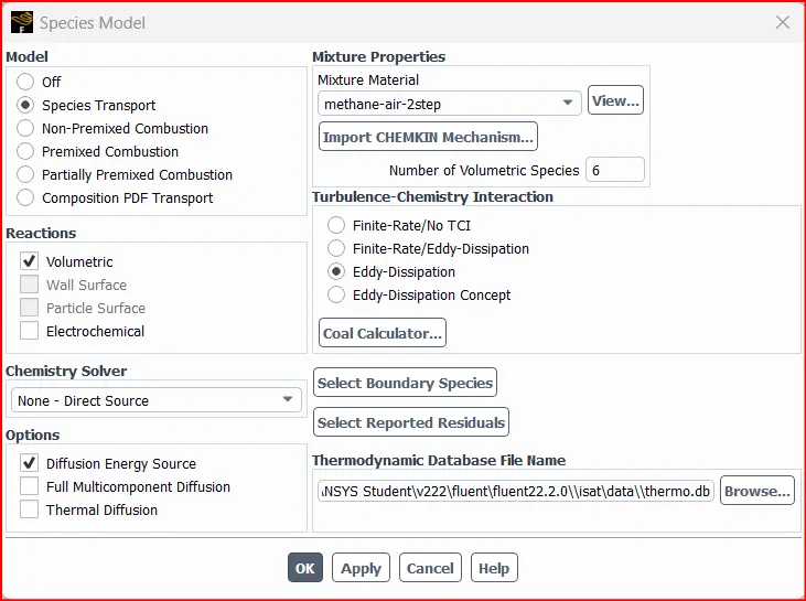
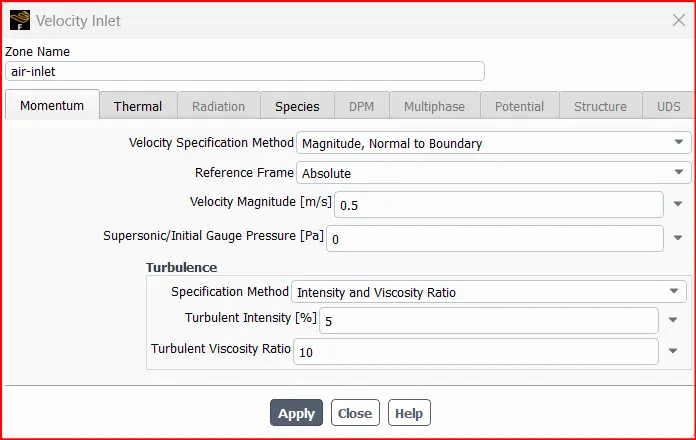
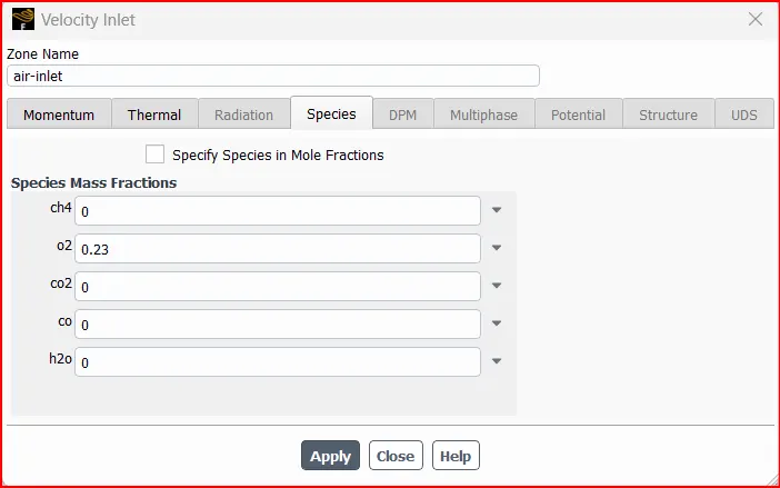
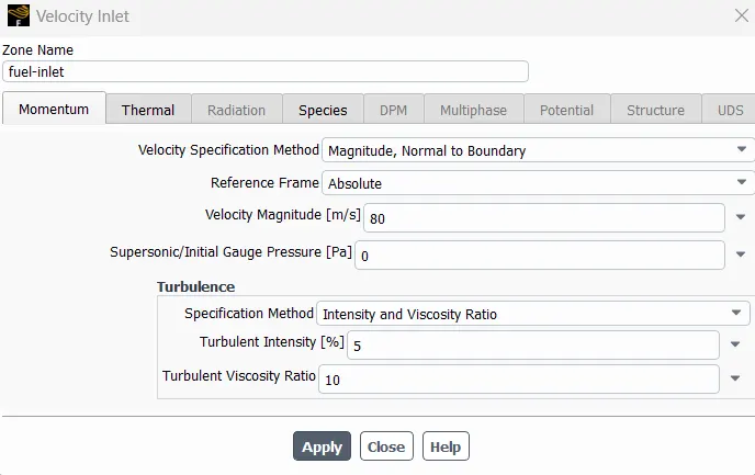
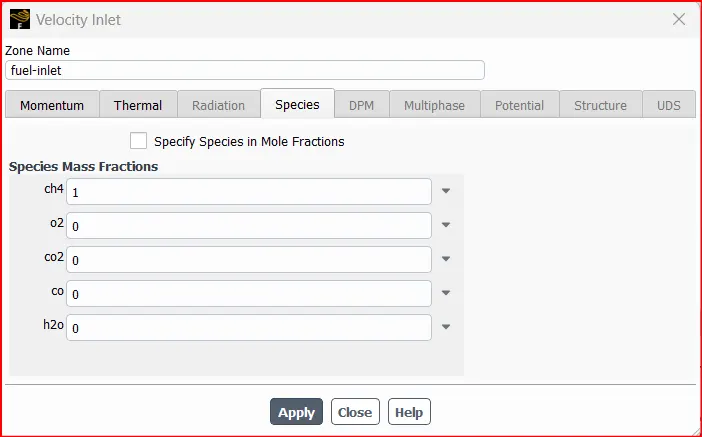
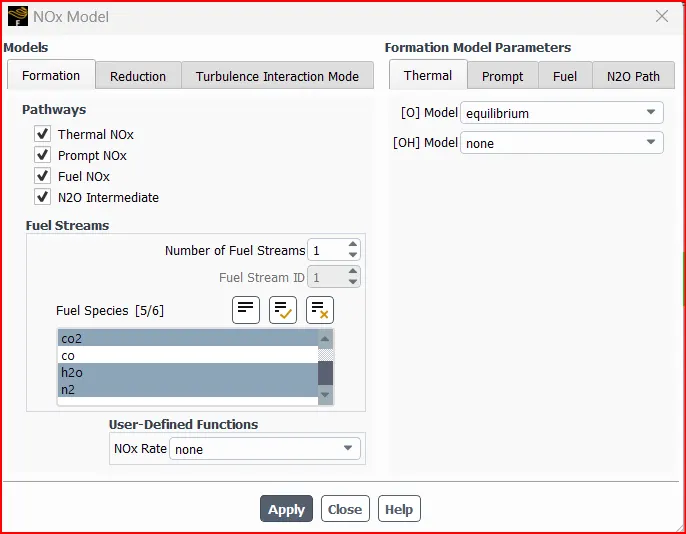
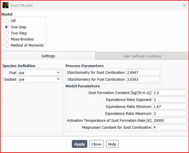
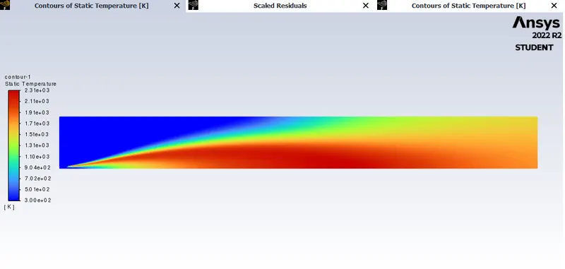
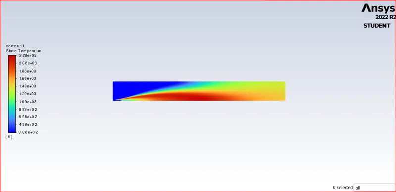
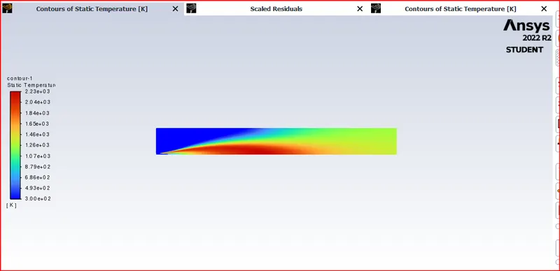
Now we can Initialise the model Run th esimulation and create contour plots of temperature distribution.
Part I
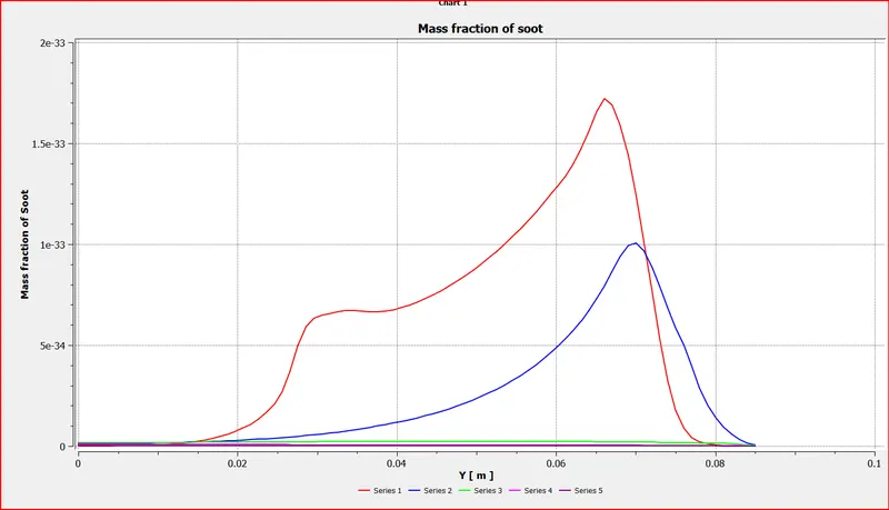
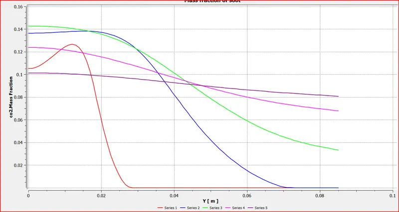
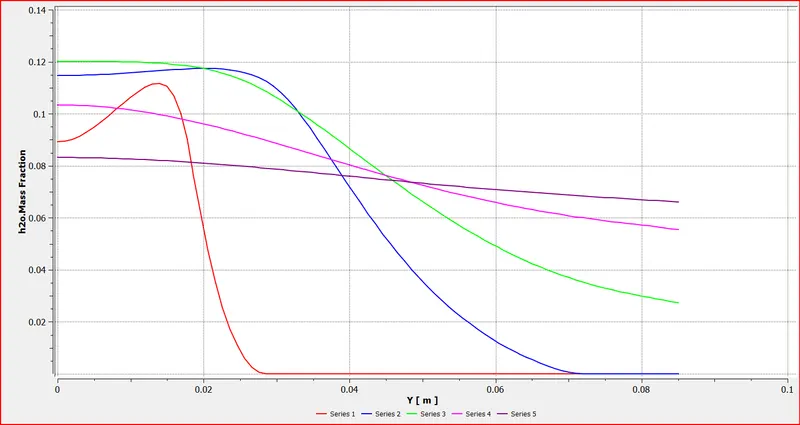
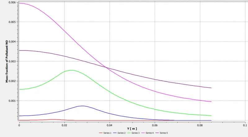
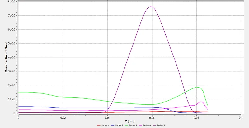
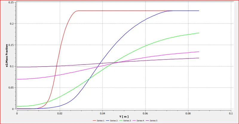
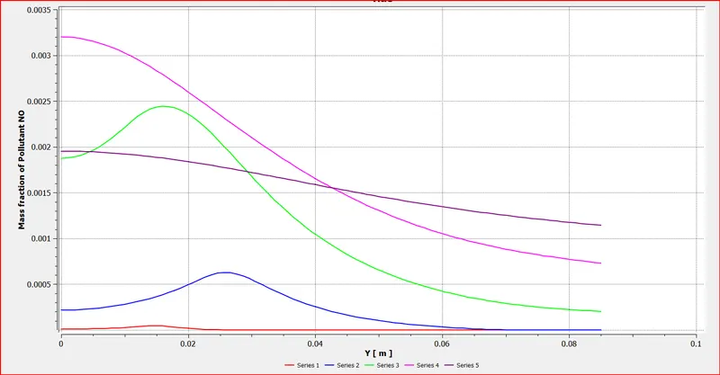
Perform a combustion simulation on the combustor model and plot the variation of the mass fraction of the different species’ in the simulation using line probes at different locations of the combustor as shown in Fig. You need to plot for CO2, H2O, CH4, N2, O2, NOx emissions & Soot formation.
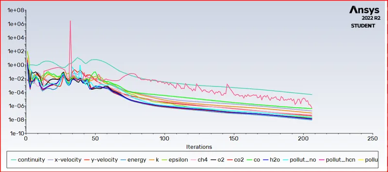
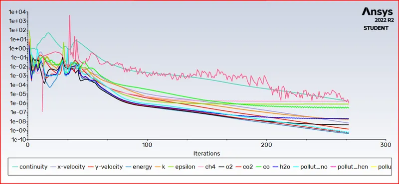
Scaled residuals..
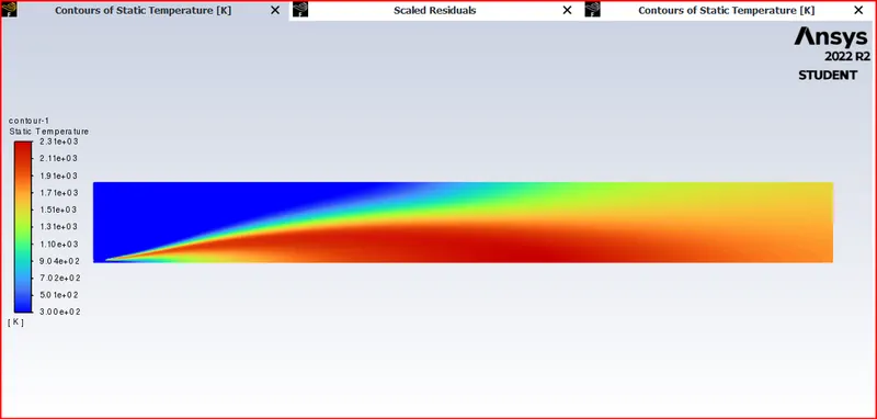
Temperature contour
Mass fraction of Soot
Mass fraction of CO2
Mass fraction of H2O
Mass fraction of CH4
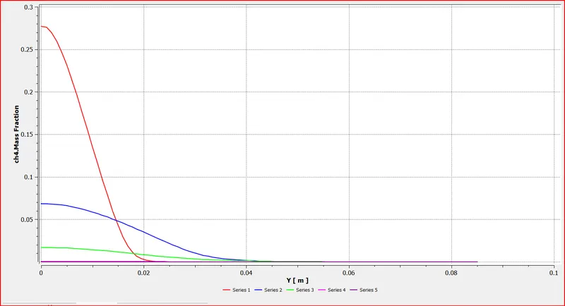
Mass fraction of N2
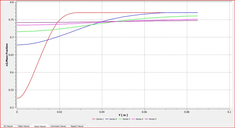
Mass fraction of O2
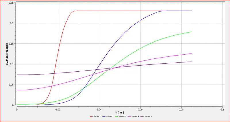
Mass fraction of NOx emissions
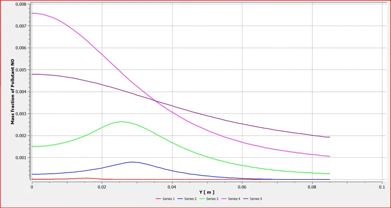
Part II
As you must have observed from the above simulation, the Nox and soot is getting formed at the outlet of the combustor. Such formation has harmful effects on the environment and humans. The stringent government norms also demand the least formation of Nox and soot and to satisfy those requirements, you need to check the effect of adding the water in the fuel.
In this part, you need to add the water content in the fuel from 5% to 30% by mole and observe the effect of it on the results. It is necessary to provide line plots and contours to prove your claim.
You can use the parametric study approach if required.
Case-1 Methane-95% and Water-5%
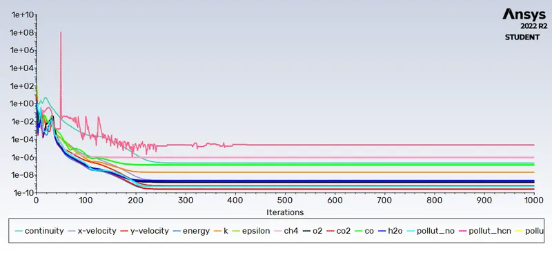
Scaled residuals..
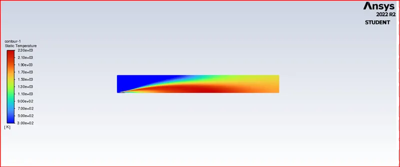
Temperature contour
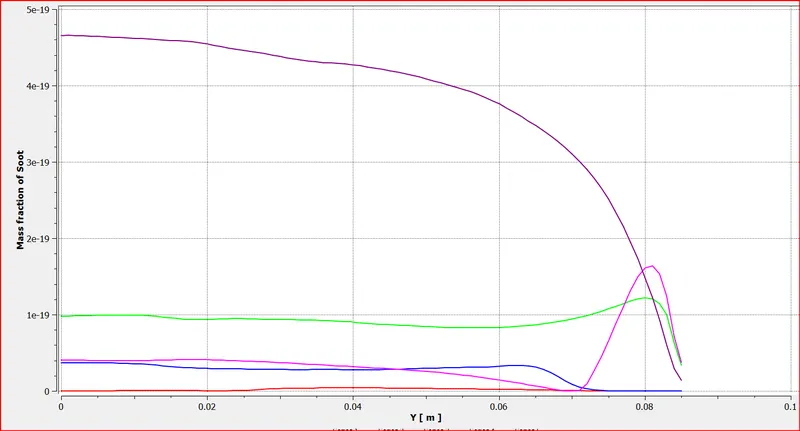
Mass fraction of Soot
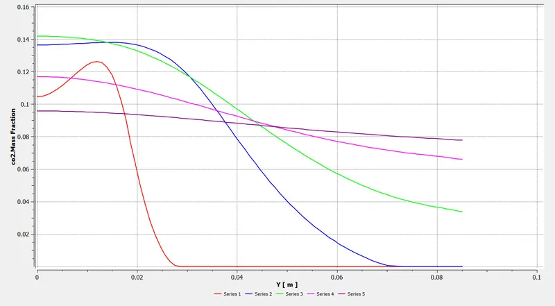
Mass fraction of CO2
Mass fraction of H2O
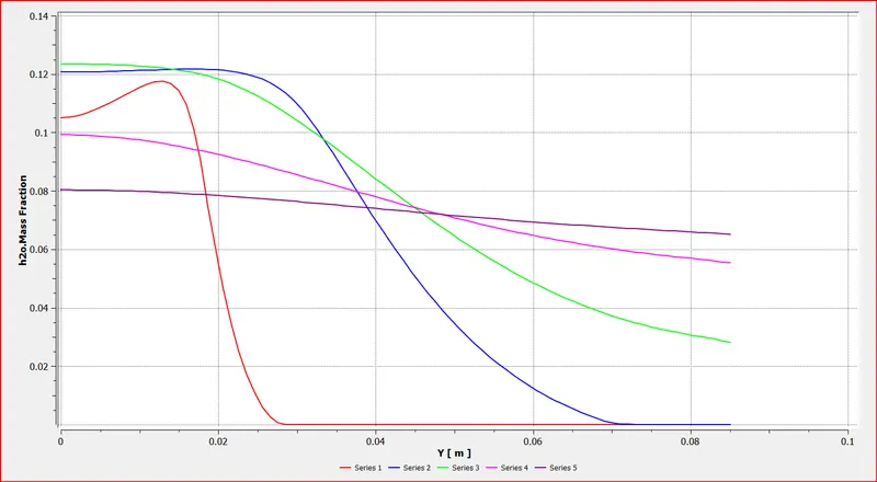
Mass fraction of CH4
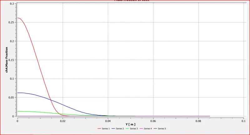
Mass fraction of N2
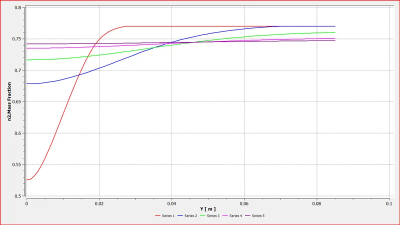
Mass fraction of O2
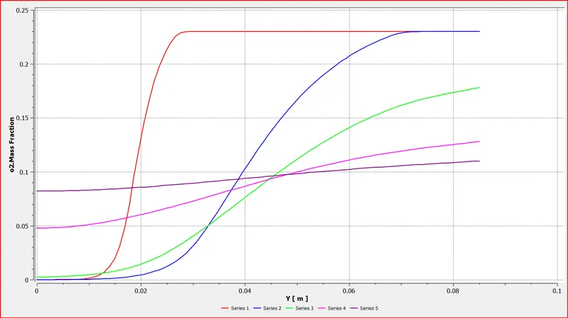
Mass fraction of NOx emissions
Case-2 Methane-85% and Water-15%
Scaled residuals..
Temperature contour
Mass fraction of Soot
Mass fraction of CO2
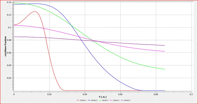
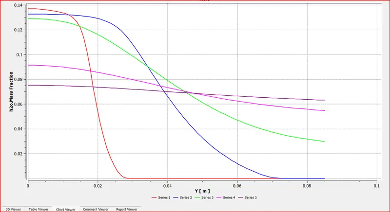
Mass fraction of H2O
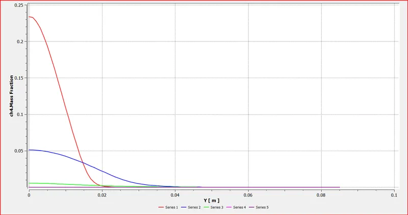
Mass fraction of CH4
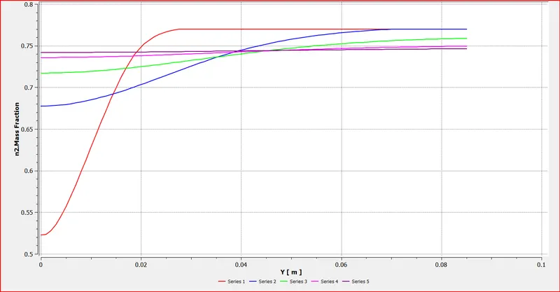
Mass fraction of N2
Mass fraction of O2
Mass fraction of NOx emissions
Case-3 Methane-70% and Water-30%
Scaled residuals..
Temperature contour
Mass fraction of Soot
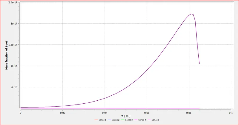
Mass fraction of CO2
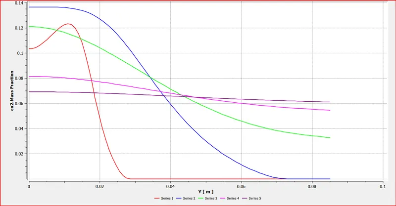
Mass fraction of H2O
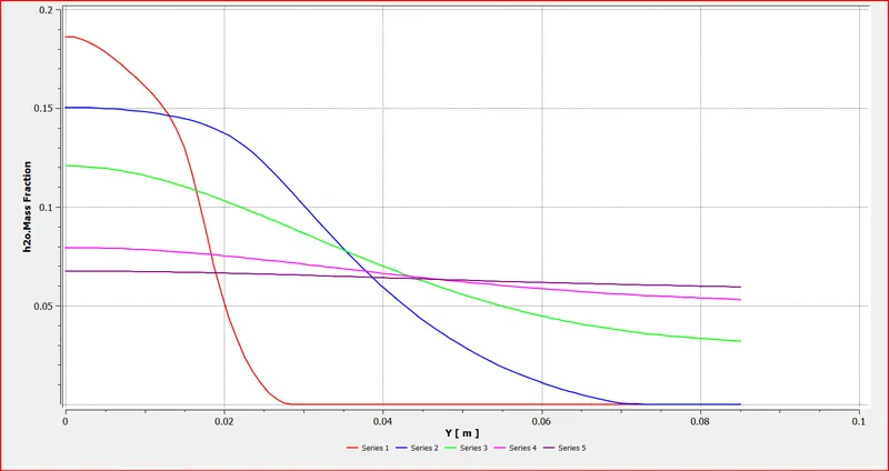
Mass fraction of CH4
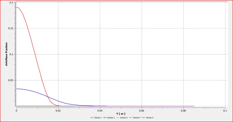
Mass fraction of N2
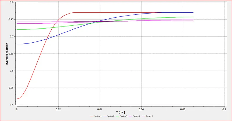
Mass fraction of O2
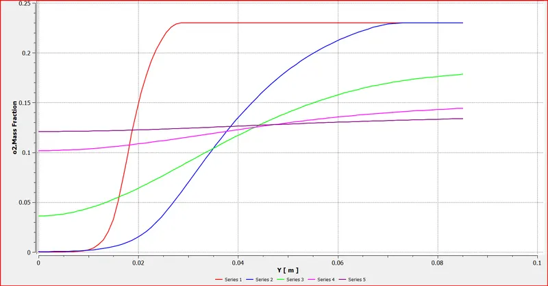
Mass fraction of NOx emissions
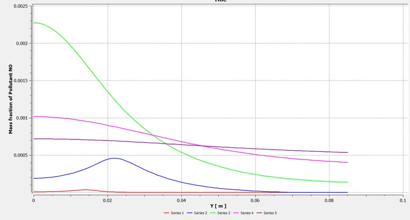
Conclusions
Simulation of combustion process is carried out using the eddy disiipation model.
Temperature contouur plots are generated for each case.
Mass fractions of pollutants like soot, ch4, co2, nox...etc are plotted.