Week 10 - Simulating Combustion of Natural Gas.
Simulating Combustion of Natural Gas
Aim
Combustion simulation of natural gas inside a burner using Ansys Fluent
Objective
- To study combustion phenomena for the whole domain.
- To study Eddy's dissipation model.
- Study the reduction behavior of NOx emission and Soot formation inside the burner.
- To pre-process the geometry for the simulation.
- Select the correct element size and type for the mesh.
- TO plot the mass fraction of CO2, H2O, N2, CH4, O2, NOx, and Soot formation.
- To perform the simulation by adding water with a fuel range of 5% to 30% to lower the burner's NOX emission and Soot formation.
Theory
Opening Remarks:
Combustion is an exothermic chemical reaction of a fuel with an oxidant to the product. There are two types of combustion:
- Flame Mode: In which the thin zone of intense chemical reaction called ‘flame’ exist.
- Non-Flame Mode: In which the volumetric combustion process is exited.
The combustion simulation is performed to get the prediction of:
- Flow field and mixing characteristic.
- Temperature field.
- Species concentration.
- Particulates of pollutants.
The application of combustion modeling is been applied to various kinds of reacting flows such as Furnaces, Boilers, Process heaters, Gas turbines, Automobiles, and Rocket engines.
Computational fluid dynamics of the combustion model should be capable enough to provide information related to species concentration, volumetric generation or diffusion rate, and changes in the system parameters like enthalpy, temperature, and mixture density.
A similar model should be good enough to solve the general transport equations for fluid flows and heat transfer as well as the additional equations of combustion chemistry and chemical kinetics incorporated as per simulation environment details.
Chemical Kinetics is part of the combustion phenomena, which is the study of the entire reaction mechanism subjected to different operating conditions.
Types of combustion simulation in Ansys Fluent
Based on Mixing:
Non-Premixed Combustion – This type of combustion occurs when oxidizer and fuel mixture enters the reaction zone in a distinct stream or are not initially mixed. Example: Diesel Engine.
Pre-Mixed Combustion – Fuel and oxidizers are mixed at the molecular level before the combustion, for Example Carburetor.
Partially Pre-Mixed Combustion – It’s between non-premixed and pre-mixed combustion where the fuel and oxidizer are partially pre-mixed at a non-uniform ratio before combustion.
Based on Phase:
Fluid Phase – Volumetric reaction takes place in the fluid region.
Wall – Combustion takes place on the surface. Example: Evaporation.
Particles – Combustion takes place on the surface of the particle. Example: Coal combustion.
Porous Region – Combustion takes place inside the pores. This type of reaction usually takes place at high-pressure drop regions.
Combustion Source Calculation
Finite Rate Chemistry:
This model derives and solves all ODEs. This results in an accurate solution but depends on the species involved, in turn, is proportional to the computation time to solve ODEs.
Mixing-Based Model
Eddy Dissipation Model:
In this model, combustion takes place in the presence of turbulence. Hence the requirement of a heat source to initiate combustion is not needed. Applicable on Non-Premixed fuel mixture.
Finite Rate Eddy Dissipation Model:
It’s a combination of finite rate chemistry and eddy dissipation models. In this model, the Kinetic rate is calculated in addition to the reaction rate calculated from the eddy dissipation model.
The slowest reaction is chosen from –
If turbulence is low, the species mixing rate is low and limits the reaction rate.
If turbulence is high, the kinetic rate is low and limits the reaction rate.
Procedure
Problem Setup
- (1) Geometry
Files → Space Claim Options → Units
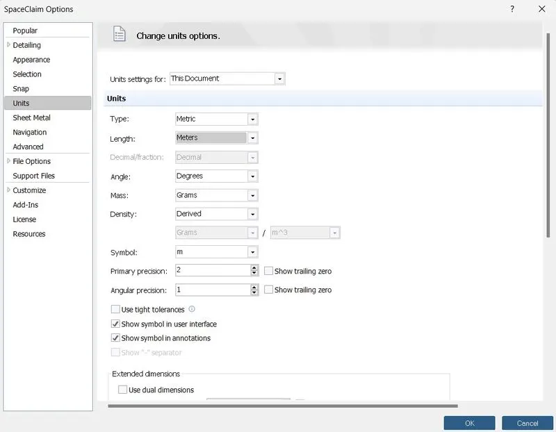
The below steps show the procedure for importing the geometry into Space-Claim and performing the necessary tasks to obtain the required simulation-ready geometry.
GEOMETRY:
- The model is imported into SpaceClaim.
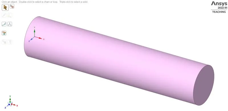
- Then the parts are combined using to combine the tool in Ansys fluent.
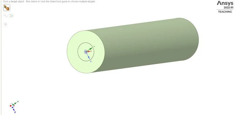
- The plane is created along the three axes and splits the body of the 3D model.
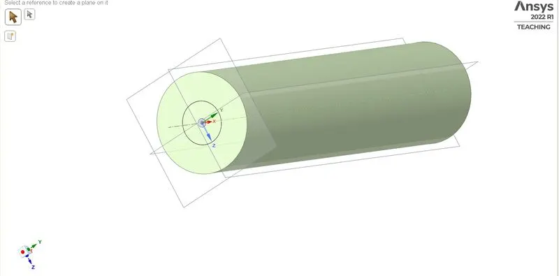
- Then the body is split into half along the z-axis.
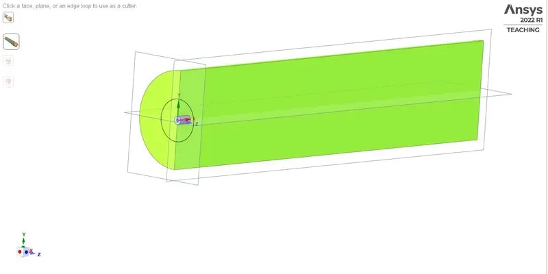
- Then the body is again split into half using the split body tool along the y-axis.
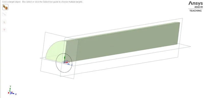
- Then the face of the model is copied and pasted into the new workspace in space claim.
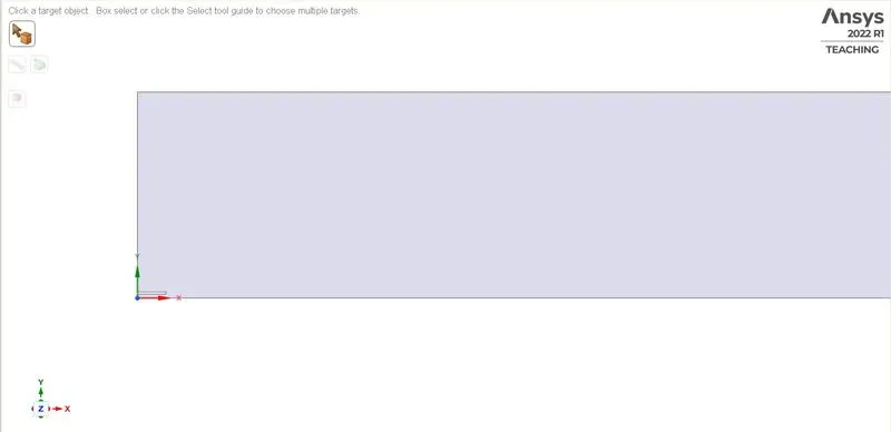
Mesh Generation
Right Click → Insert → Named Selection, As follows
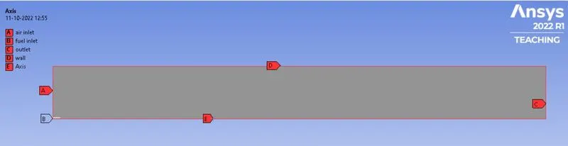
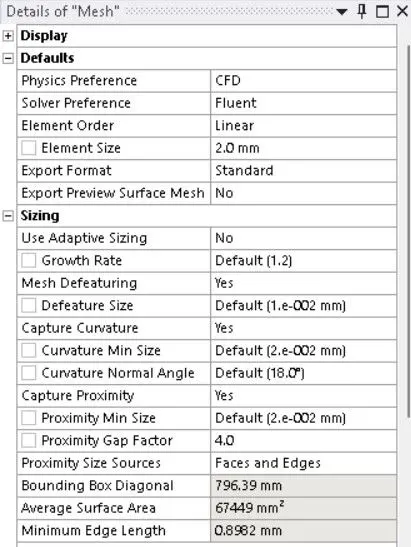
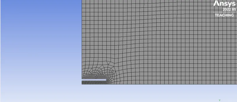
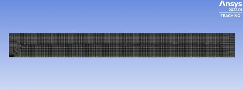
- The model is discretized into small elements of size 2mm and capture proximity is turned on and the number of cells across the gap is 4
- The final meshed model will look like the image below
Mesh Quality
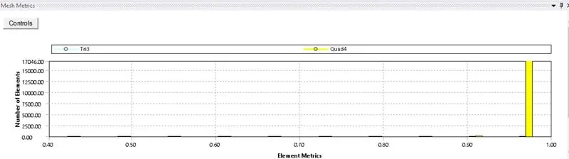
Element Quality

SETUP:
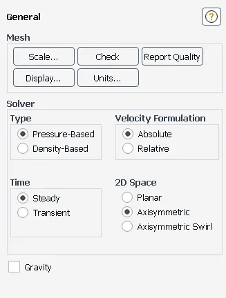
GENERAL:
-
- General → Solver → Pressure-based → Time→ Steady State → 2D Space → Axis-symmetry → Velocity Formulation → Absolute
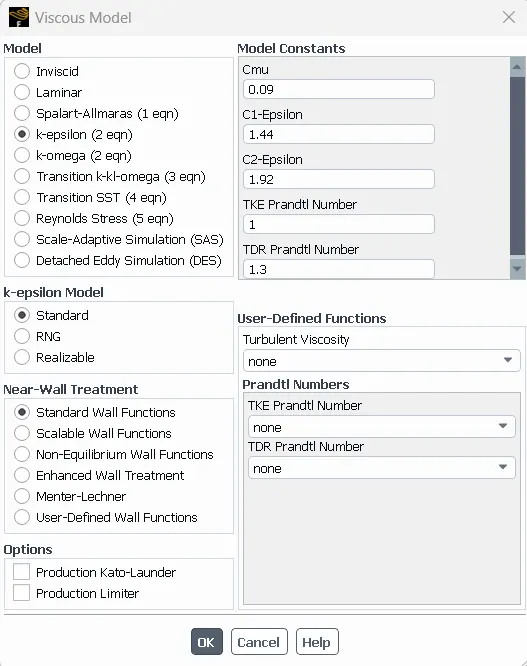
- Models → Viscous → K-epsilon → Standard → Standard Wall Function
Energy → Energy equation → On

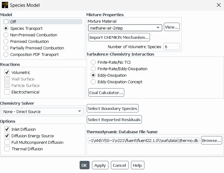
Species →
- Model – species transport
- Reactions – volumetric
- Options – inlet diffusion, diffusion energy source.
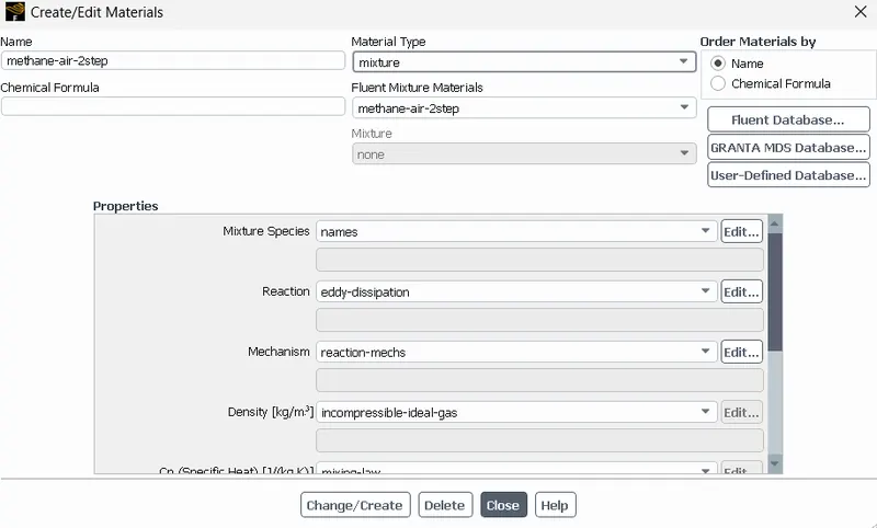
- Mixture material – methane-air 2 step
- Turbulence chemistry interaction – eddy dissipation.
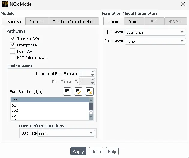
NOx Model →
- Pathways – thermal, prompt NOx
- Fuel species – CH4
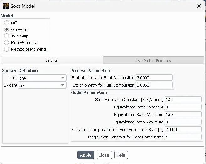
Soot Model →
- Model – one step
- Fuel – CH4
- Oxidant – O2
Material →
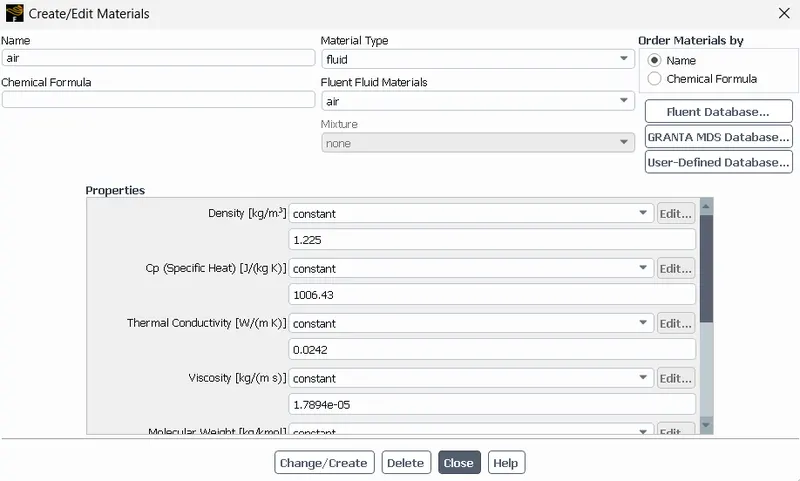
Fluid → Air →
MIXTURE MATERIAL:
- Add New → Fluent Database → Methane-Air-2Step →
Cell Zone Conditions → fff_surface → Fluid → User-material
Boundary Conditions
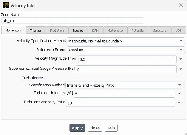
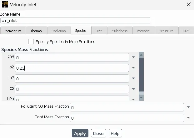
Air-Inlet →
- Velocity – 0.5m/s
- Temperature – 300k
- O2 – 0.23
Momentum
Species
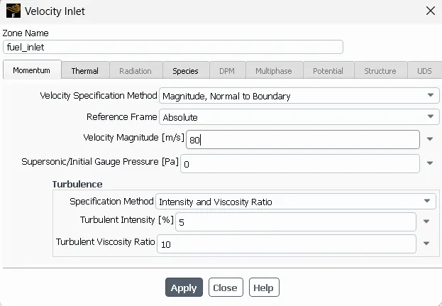
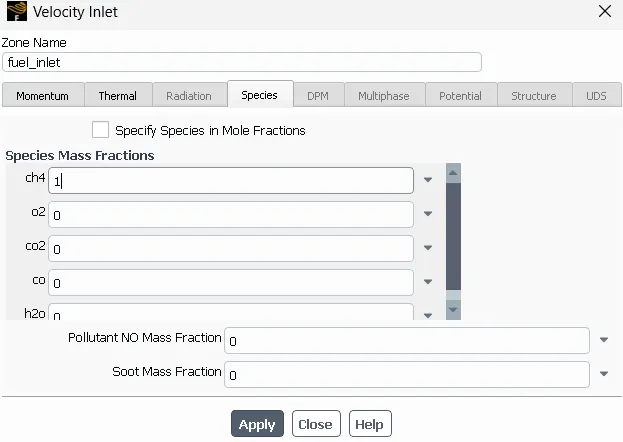
Fuel-Inlet →
- Velocity – 80m/s
- Temperature – 300k
- CH4 - 1
Momentum
Species
- Outlet (Gauss Pressure=1 atm)
- Wall_fff-surface → Wall Motion → Stationary → Shear Condition → No Slip
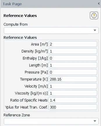
- Reference Values →
- Method → Scheme → Coupled
- Results → Create → Line →
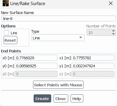
- Solution → Definition →
- Surface Report → Weighted Average → Mass Fraction of NO pollutant → Field Variable = monitor-Line
- Surface Report → Weighted Average → Mass Fraction of Soot→ Field Variable = monitor-Line
Initialize Solution → Hybrid

Part 1 :
To perform a combustion simulation on the Burner model and plot the variation of the mass fraction of the different species in the simulation.
Result
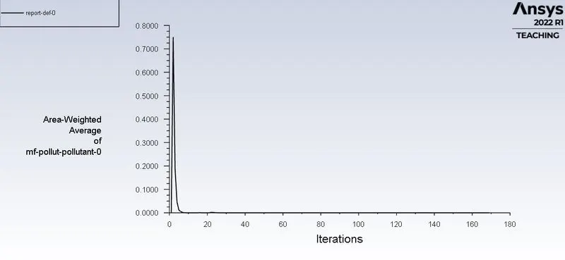
Residual Plot
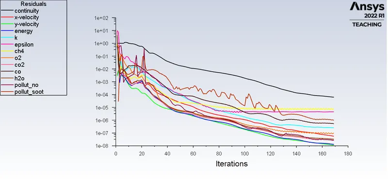
TEMPERATURE CONTOUR:
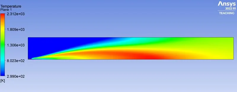
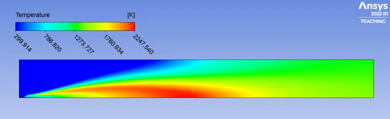
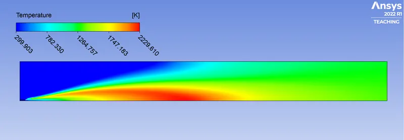
From the temperature contour, we can say that the temperature is higher in the regions where the air-fuel mixture takes place.
Line Probe Geometry
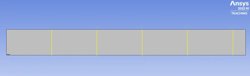
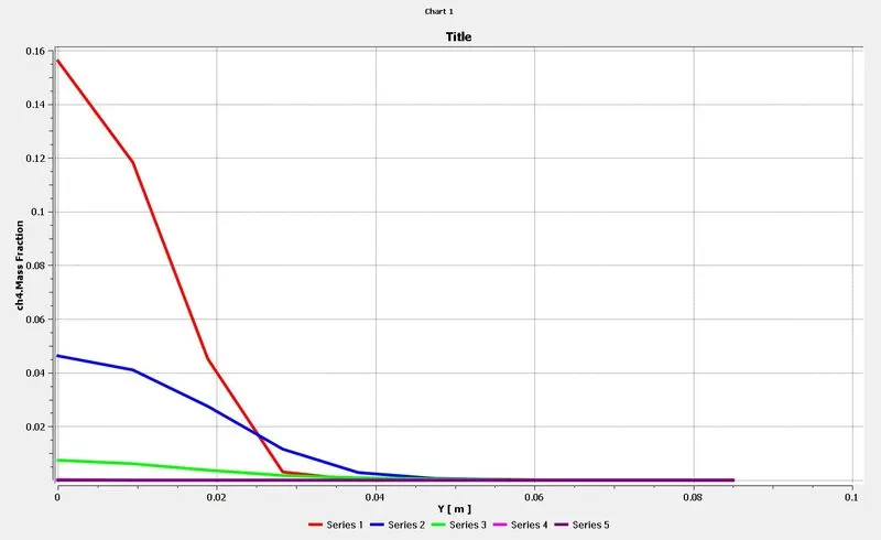
we are considering five line probes at distances of 0.15,0.30, 0.45, 0.60, and 0.75m respectively.
CHART LEGEND
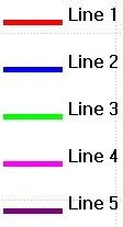
Mass Fraction Contours & Plots
CH4:
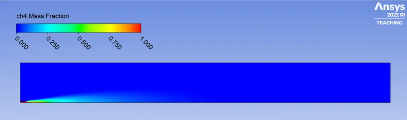
From this contour, we can say that the CH4 mass fraction is higher near the fuel inlet where the fuel is being injected and decreases once the combustion takes place.
CHART:
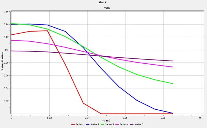
Co2:
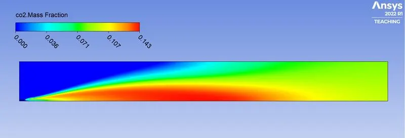
From this contour, we can say that the CO2 mass fraction is higher in the regions where the temperature is higher.
CHART:
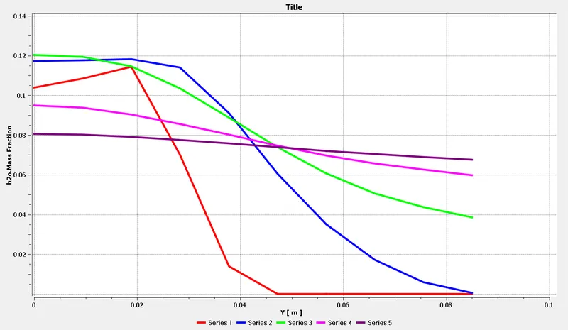
H2o:
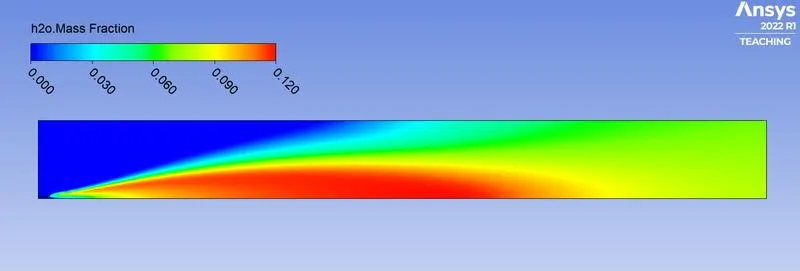
From this contour, we can say that the H2O mass fraction is higher in the regions where the CO2 mass fraction is higher.
CHART:
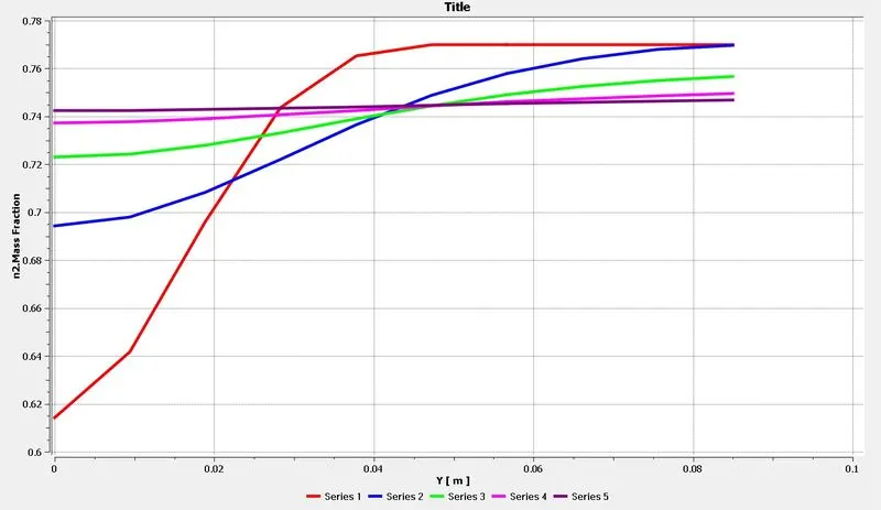
N2
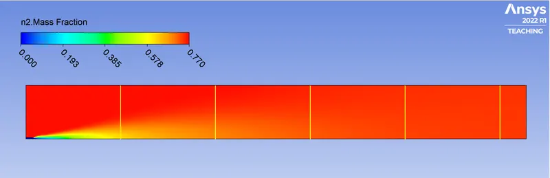
From this contour, we can say that the N2 mass fraction is uniformly distributed across the combustor.
CHART:
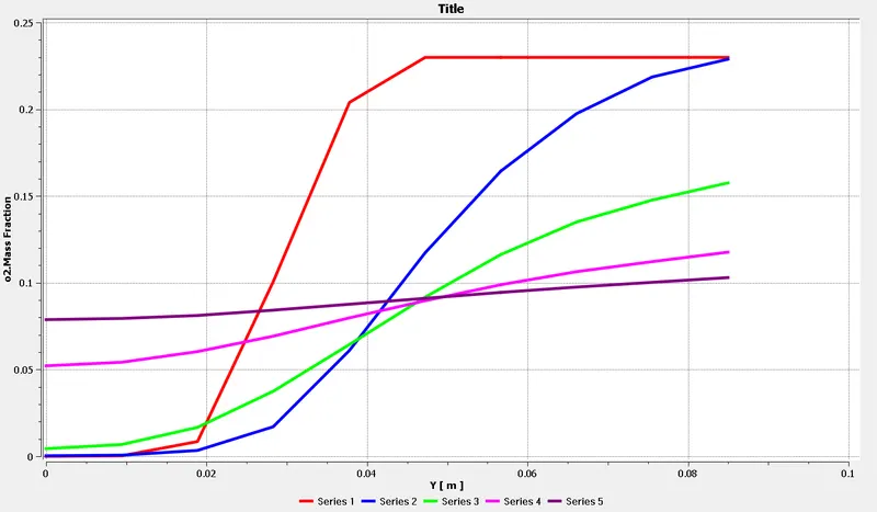
O2
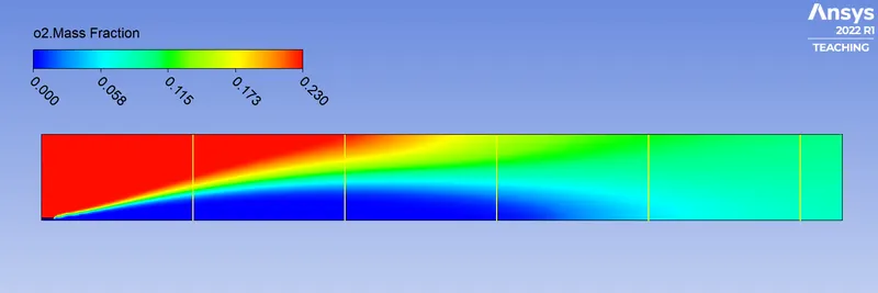
From this contour, we can say that the O2 mass fraction is higher near the air inlet where the air is being injected.
CHART:
NOx Emission:
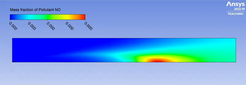
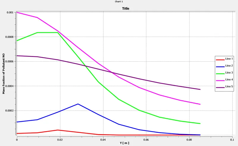
From this contour, we can conclude that the mass fraction of NO is higher at the outlet of the combustor. [As I used precision as 2 and fixed it is showing values as zero in contour]
CHART:
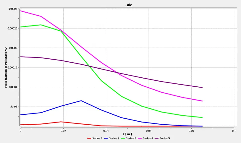
Outlet:

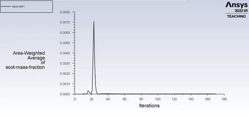
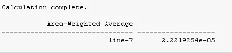
Soot Formation:
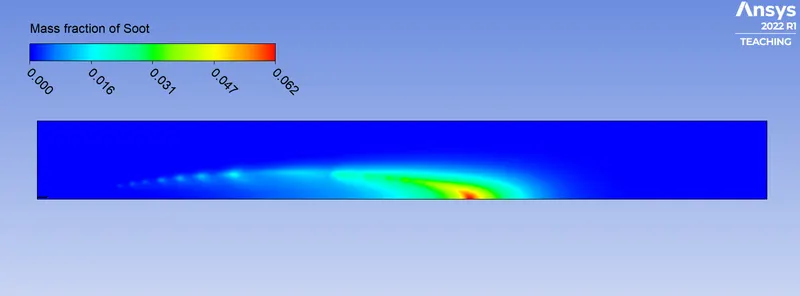
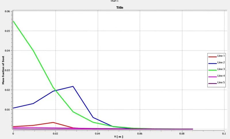
From this contour, we can conclude that the soot mass fraction is higher at the outlet.
CHART:
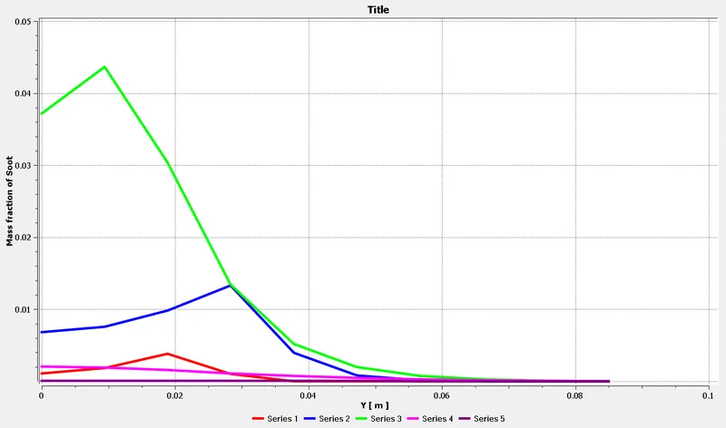
Outlet:
Part 2
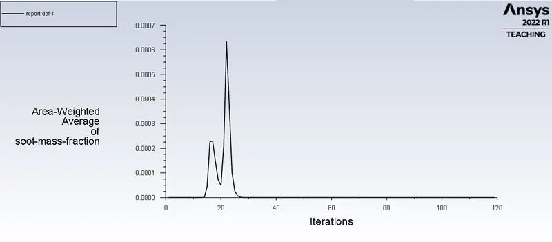
To perform a combustion simulation on the Burner model and add water content in the fuel from 5% to 30% by mole. For which observe the effect of it on the results. Also, provide line plots and contour to prove your claim.
Case 1
WATER 5%
RESULTS:
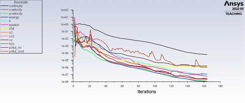
RESIDUAL:
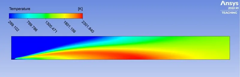
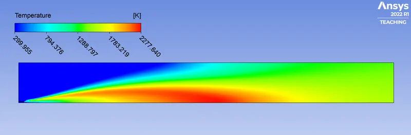
TEMPERATURE CONTOUR:
NOx:
MASS FRACTION:
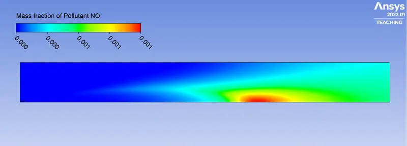
CHART:
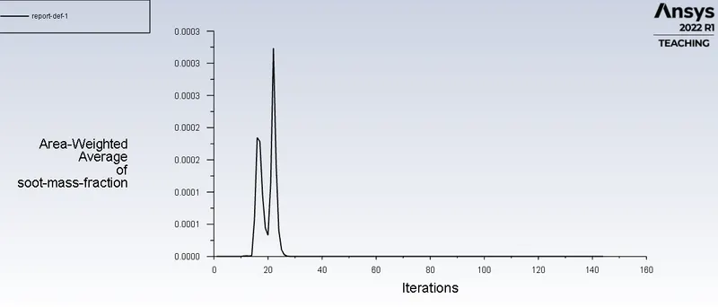
Graph:
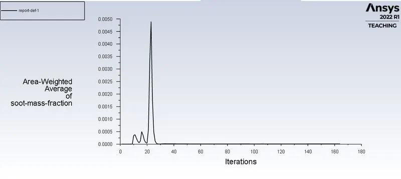
SOOT:
MASS FRACTION:
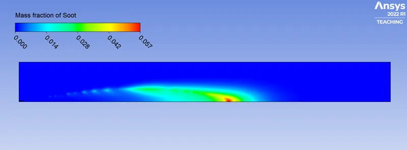
CHART:
Graph:
Case 2
WATER 15%
RESULTS:
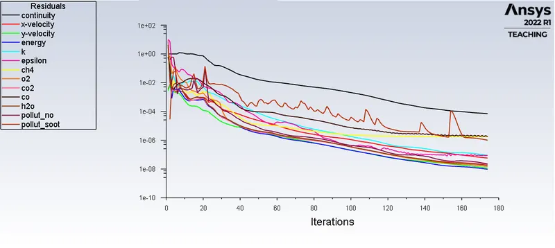
RESIDUAL:
TEMPERATURE CONTOUR:
NOx:
MASS FRACTION:
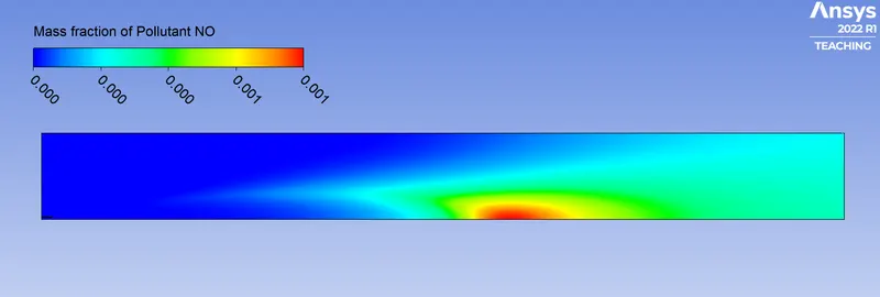
CHART:
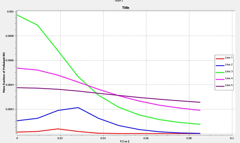
Graph:
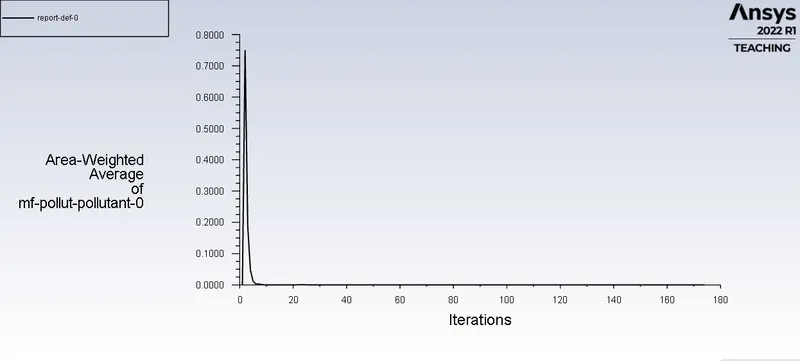
SOOT:
MASS FRACTION:
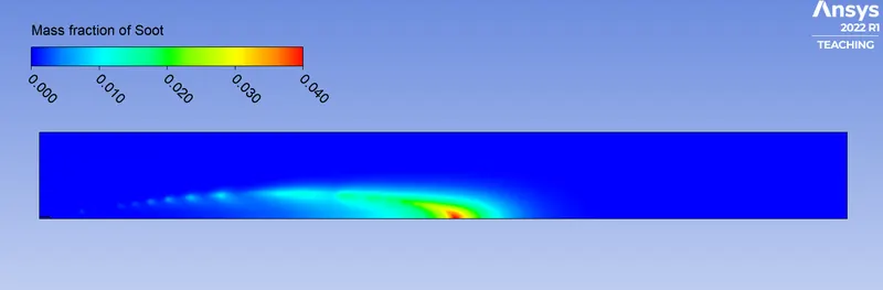
CHART:
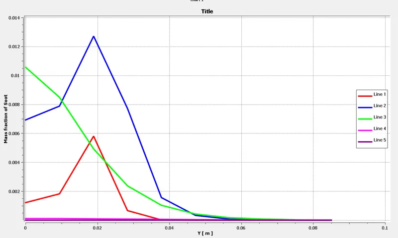
Graph:
Case 3
WATER 25%
RESULTS:
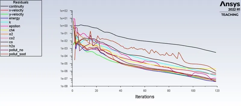
RESIDUAL:
TEMPERATURE CONTOUR:
NOx:
MASS FRACTION:
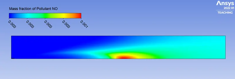
CHART:
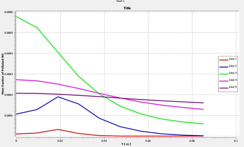
Graph:
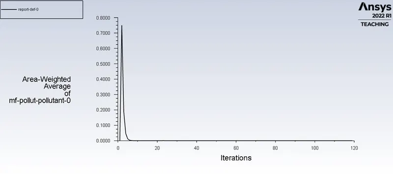
SOOT:
MASS FRACTION:
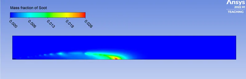
CHART:
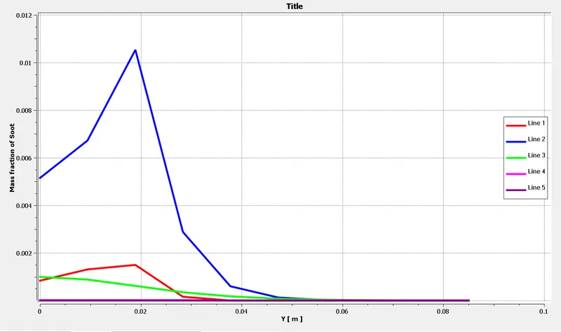
Graph:
Case 4
WATER 30%
RESULTS:
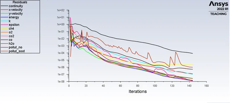
RESIDUAL:
TEMPERATURE CONTOUR:
NOx:
MASS FRACTION:
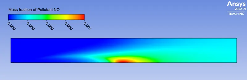
CHART:
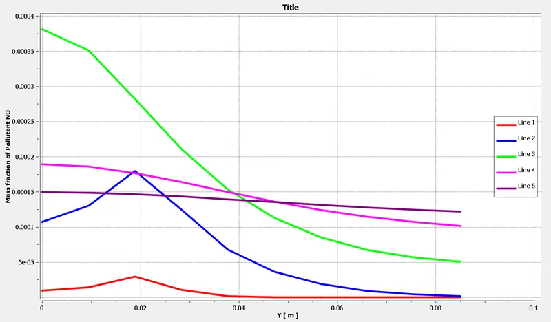
Graph:
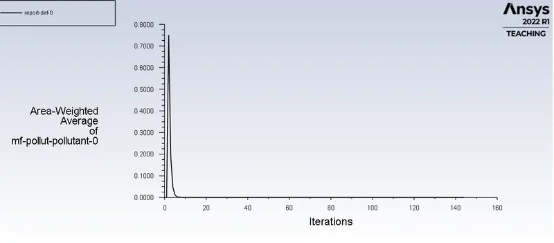
SOOT:
MASS FRACTION:
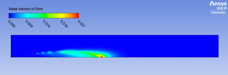
CHART:
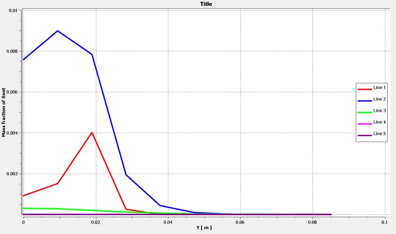
Graph:
Parametric Study Data

B and C is inputs D,E,F,G,H,I,and J is an outputs
| report-def number | Title |
| 0 | NOx |
| 1 | Soot |
| 2 | ch4 |
| 3 | o2 |
| 4 | Co2 |
| 5 | h2o |
| 6 | co |
| 7 | n2 |
Conclusion :
In this project, the mass fraction of pollutants from NOx and Soot emissions are predicted using Ansys Fluent. The results obtained from the simulation show:
- The temperature drops as we add water to the fuel from 5% to 30%.
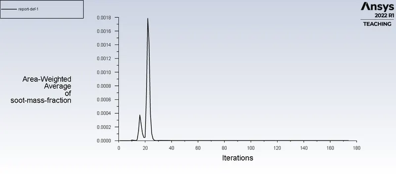
- The mass fraction of NOx emission and Soot decreases as we add water to the fuel by 5% to 30%. And this can be noticed in the parametric study data.
- Also, from the data study, it can be seen that the mass fraction of Co2 is decreasing as the water percentage is increasing.
- The mass fraction of N2 is almost constant for all cases, which means the flame instability for the burner is almost constant for all the cases of combustion.
- After checking the mass fraction of soot formation, it’s evident that for all cases results in an unbalanced. But the amount of soot formation is significantly lower and is nearer to an outlet of the burner.
Reference
1. https://www.sciencedirect.com/science/article/pii/S1876610217337724
2. https://link.springer.com/article/10.1007/s00773-015-0303-8