Challenge

Week 10 - Simulating Combustion of Natural Gas.

SSugumar P20 Sept 2022

Part I

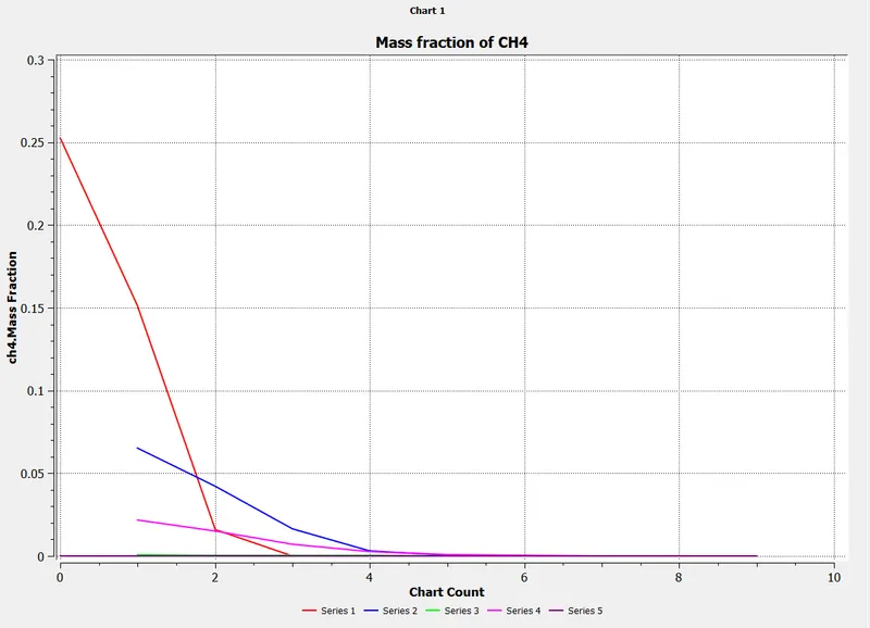
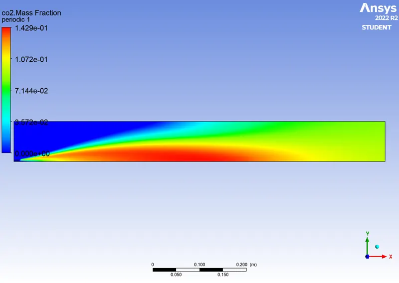
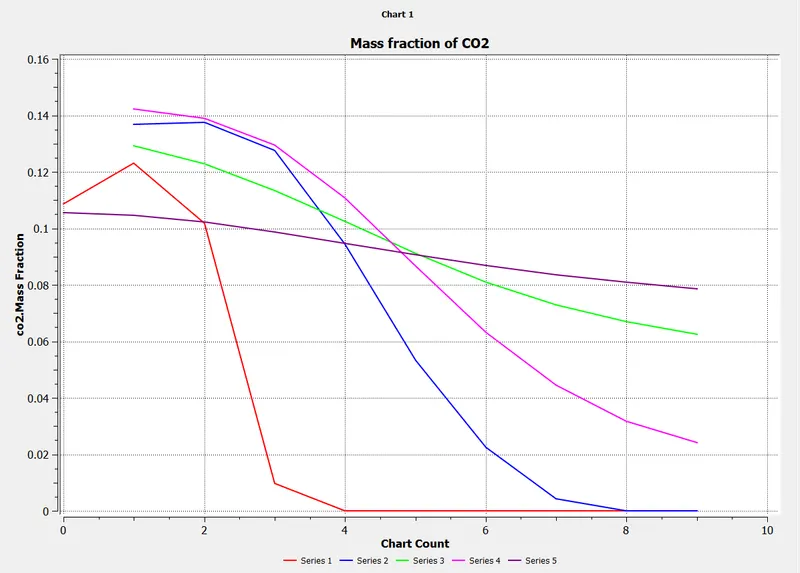
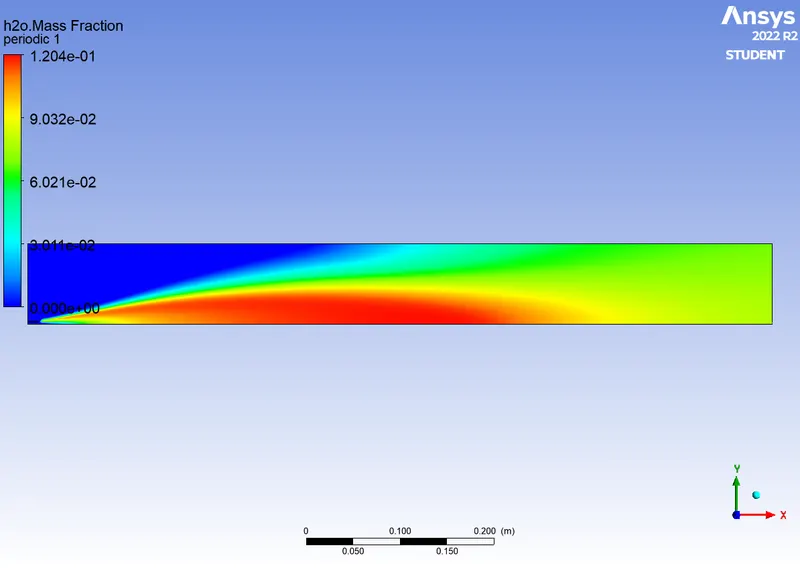
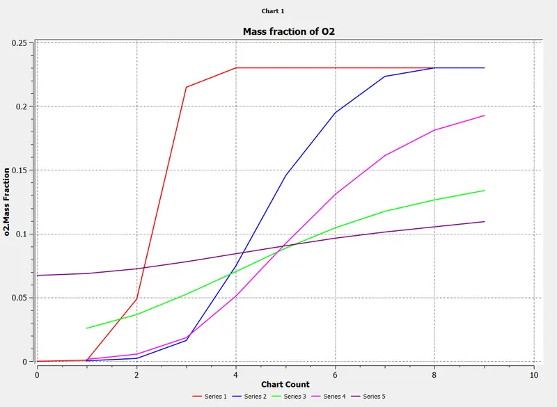
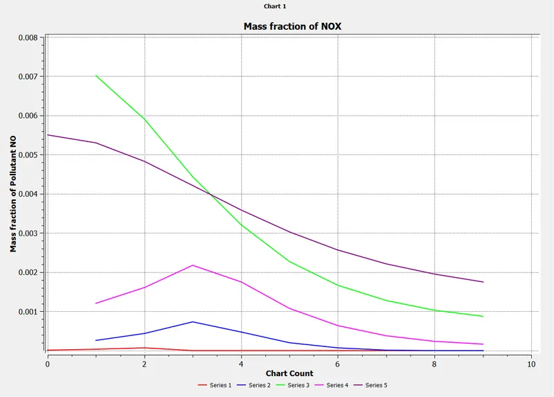
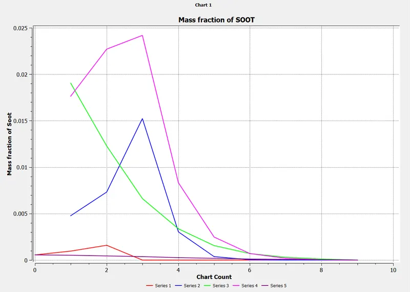
Perform a combustion simulation on the combustor model and plot the variation of the mass fraction of the different species’ in the simulation using line probes at different locations of the combustor as shown in Fig. You need to plot for CO2, H2O, CH4, N2, O2, NOx emissions & Soot formation.

Part II

As you must have observed from the above simulation, the Nox and soot is getting formed at the outlet of the combustor. Such formation has harmful effects on the environment and humans. The stringent government norms also demand the least formation of Nox and soot and to satisfy those requirements, you need to check the effect of adding the water in the fuel.

In this part, you need to add the water content in the fuel from 5% to 30% by mole and observe the effect of it on the results. It is necessary to provide line plots and contours to prove your claim.

You can use the parametric study approach if required.

SOLUTION

AIM

To perform a combustion simulation on the combustor model.

Objective

Part I

Perform a combustion simulation on the combustor model and plot the variation of the mass fraction of the different species’ in the simulation using line probes at different locations of the combustor as shown in Fig.
You need to plot for CO2, H2O, CH4, N2, O2, NOx emissions & Soot formation.

Part II

As you must have observed from the above simulation, the Nox and soot is getting formed at the outlet of the combustor. Such formation has harmful effects on the environment and humans. The stringent government norms also demand the least formation of Nox and soot and to satisfy those requirements, you need to check the effect of adding the water in the fuel.
In this part, you need to add the water content in the fuel from 5% to 30% by mole and observe the effect of it on the results. It is necessary to provide line plots and contours to prove your claim.

Introduction

Combustion

Combustion involves chemical reactions converting fuel and oxygen to combustion products with light and heat energy. It involves fluid flow, consumption and generation of species by chemical kinetics and heat transfer ( convection and radiation).
Combustion becomes more complex because of phenomena of flame propagation, slow or fast ignition, explosions, slow ignition, correct fuel to oxidizer ratios, phase change for liquid fuel,and so forth depend in subtle ways on the conditions under which combustion takes place.

Application of Combustion Modeling

Burners: LPG gas stoves, Furnaces, Boilers, Gasifier etc.
Engine : Petrol and diesel engines
Gas turbine combustor: Power plant steam turbine, air-craft gas turbine combustor etc.
Safety: protection from fires, explosions or blast etc.
Emission controls: Design and development of low NOx/SOx burner or combustor.

Based on mixing

Premixed combustion

In the mixing chamber, fuel and oxidizer (air) are already mixed at the molecular level before ignition or combustion
Cold reactants propagate into hot products
Rate of propagation (flame speed) depends on the internal flame structure
Much more difficult to model than non-premixed combustion problems
Turbulence distorts the laminar
Examples: SI enginer, LPG gas stove etc.

Non-premixed combustion

Separate inlet/ streams for Fuel and oxidizer (air) to the combustion chamber
Convection or diffusion of reactants from either side into a flame sheet
Turbulent eddies distort the laminar flame shape and enhance mixing
May be simplified to a mixing problem
Examples: Burner for boiler /furnaces, coal combustion, candle flame, wood fire etc.

Partially premixed combustion

In some applications, primary air (oxidizer) is mixed with fuel to form the unburnt mixture before combustion such cases are treated as partially premixed combustion.
Premixed fuel/oxidizer inlet streams

Based on Phase

Volumetric: Takes place when the fluid is in fluid phase.

Surface: Takes place on the wall.

Porous: Takes place inside pores

Eddy dissipation

Most fuels are fast burning and the overall rate of reaction is controlled by turbulence mixing.
In the non-premixed flames, turbulence slowly mixes the fuel and oxidizer into the reaction zones where they burn quickly.
In premixed flames the turbulence slowly mixes cold reactants and hot products into the reaction zones where reaction occurs rapidly. In such cases the combustion is said to be mixing-limited, and the complex and often unknown chemical kinetics can be safely neglected.
In this model, the chemical reaction is governed by large eddy mixing time scale. Combustion initiates whenever there is turbulence present in the flow. It does not need an ignition source to initiate the combustion.
This type of model is valid for the non-premixed combustion, but for the premixed flames the reactant is assumed to burn at the moment it enters the computation model, which is a shortcoming of this model as in practice the reactant needs some time to get to the ignition temperature to initiate the combustion.

GEOMETRY

The combustor step file is imported into spaceclaim and using the split body command and only a qaurter of the solid model is selected and the 3d surface is copied into a new 2-D model, where it is combined using combine command.

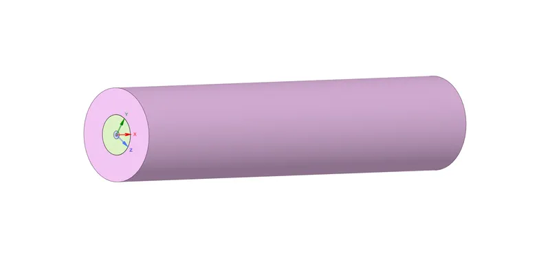
This is 3D model, we can't run simulation for entire 3D model, it will cost a lot interms of time.
So instead of 3D, We will perform simulation on 2D geometry, which is Axis-symmetric.
For 2D geomerty we have to cut 3D model in two parts, and extract 2D geometry of the quadrant portion

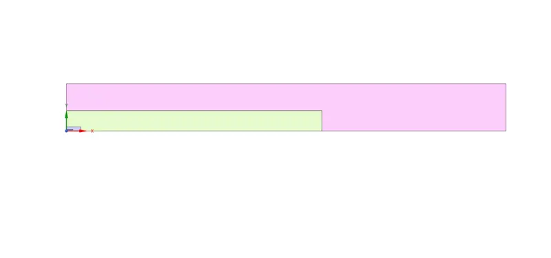
Then we copy all faces from X-Y plane and paste it in New Design
Then we paste it only in X-Y plane.
After pasting, we merge all faces by using 'combine' command and can make it a single surface.

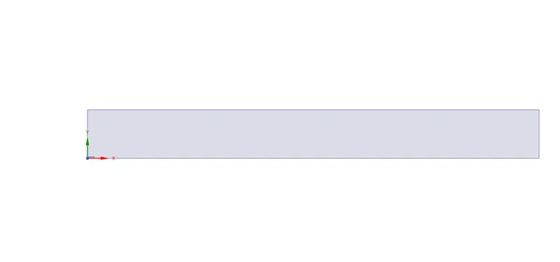
So the 2D geometry can be ready for further process

MESH

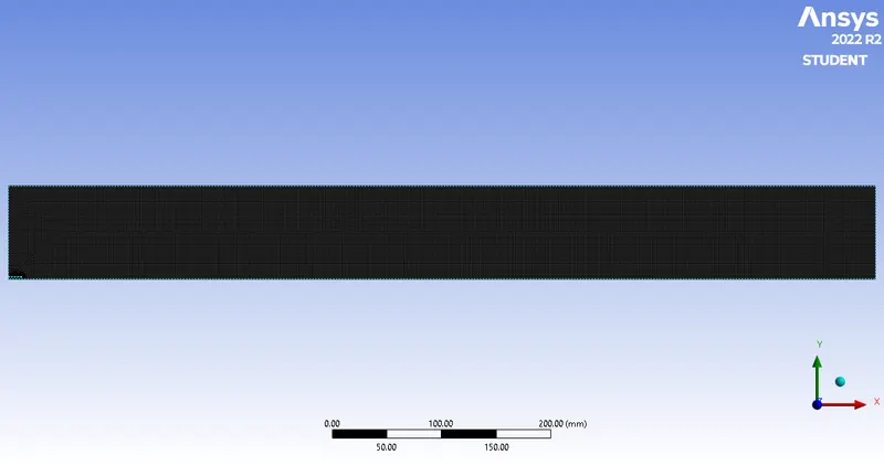
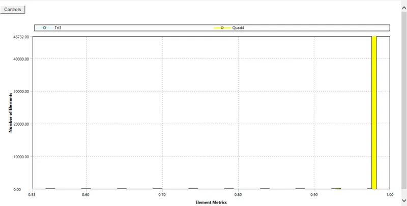
The mesh size is set to 1.2mm and the capture proximity is turned on.

Then the inlet, outlet, walls, aand axis are named.

Element size : 1.2mm

No of elements : 46981

SETUP

Solver

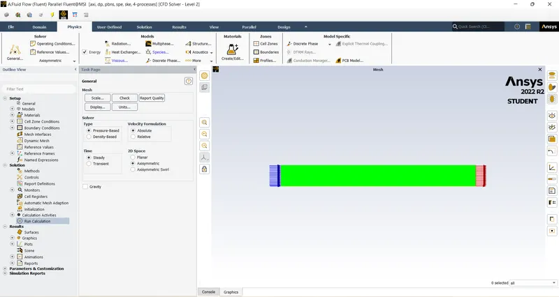
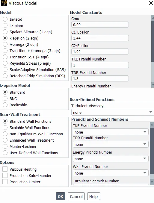
The set up begins with activating the energy equation, then the 2D space is set to axissymmetric. K-ε">εε→">→→standard→">→→standard wall function is chosen.
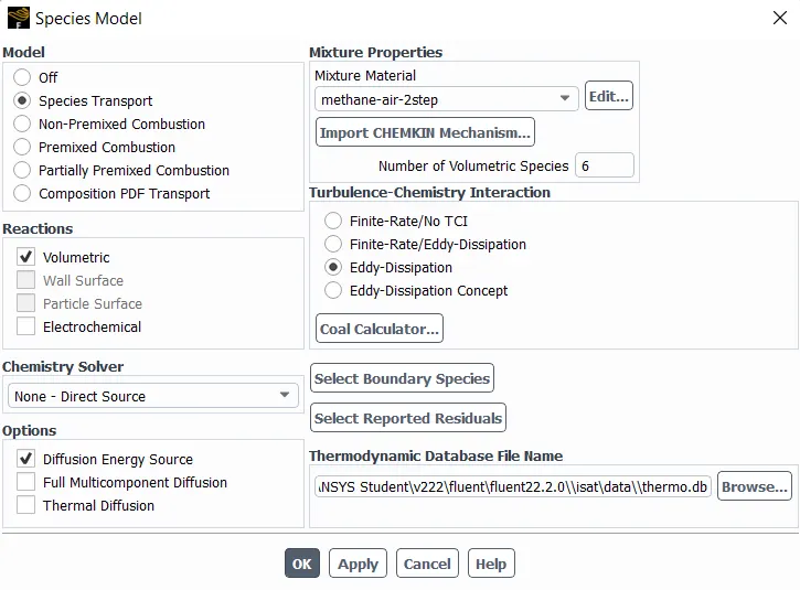
Species transport, the volumetric reaction and diffusion energy source is selected. methane-air-2step mixture model and eddy dissipation is chosen.
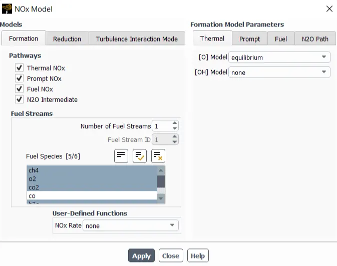
In the NOX model, all the pathways are selected and the desired species whose values needed to be calculated are selected.
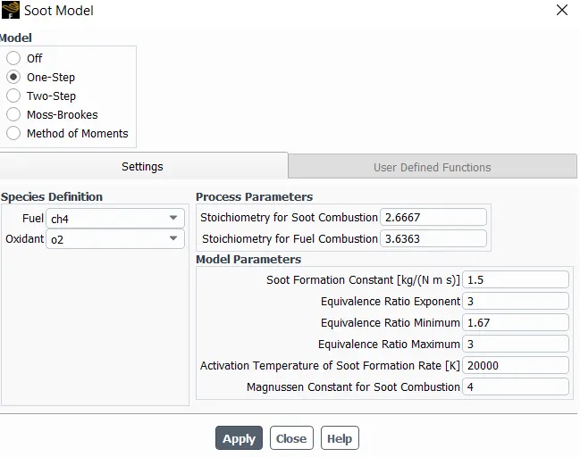
One-step soot model is chosen and CH4 is set as the fuel and O2 is set to oxidant.
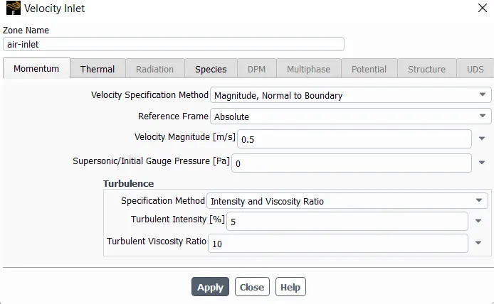
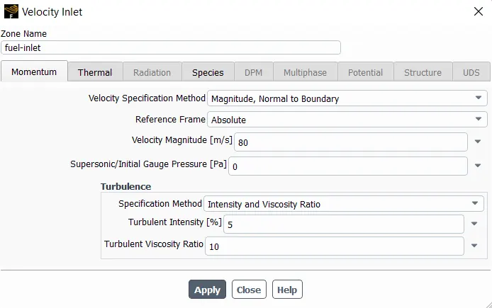
The air-inlet boundary velocity is set to 0.5m/s and for fuel is set to 80m/s.
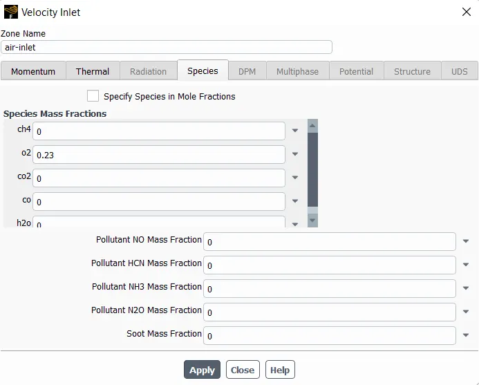
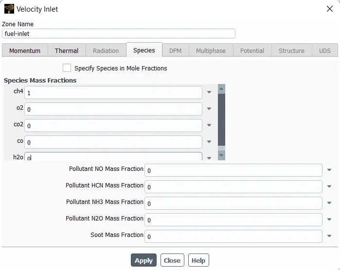
The fuel mass fraction of CH4 is set to 1 and varied accordingly and the air mass fraction is set to 0.23.
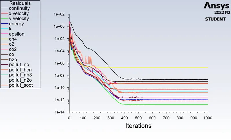
The hybrid initialisation is done and then the iterations are run for 1000iterations.

VISCOUS MODEL

SPECIES MODEL

NOX MODEL

SOOT MODEL

VELOCITY

POST-PROCESSSING

CFD-POST

PART-1

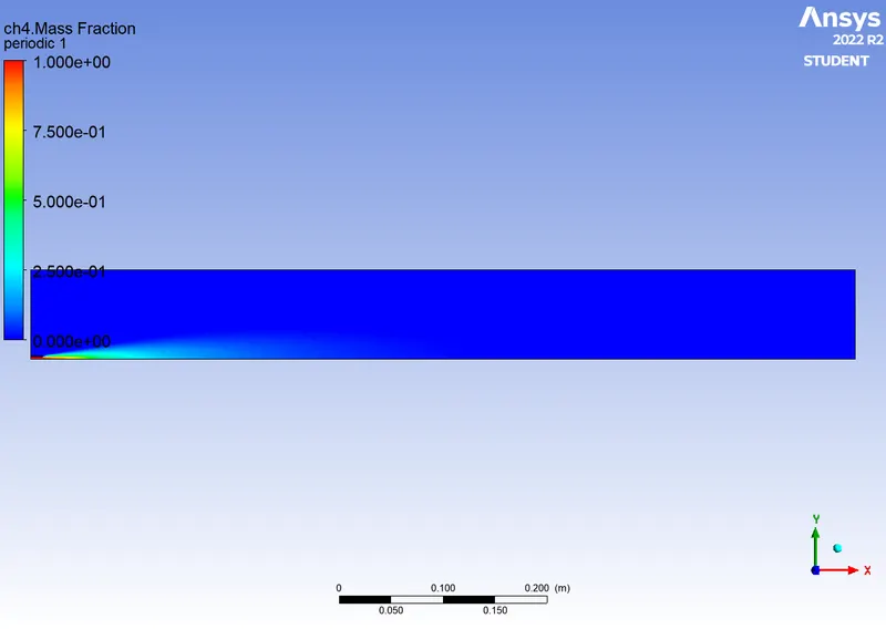
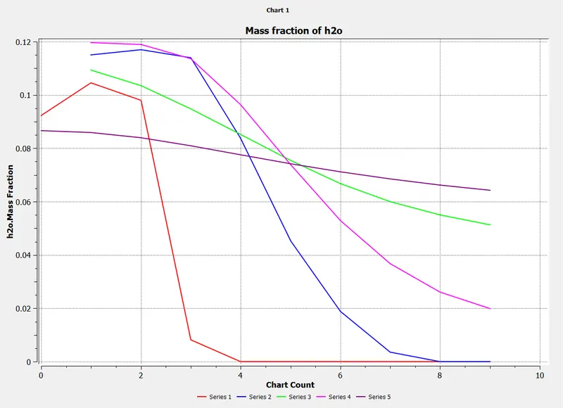
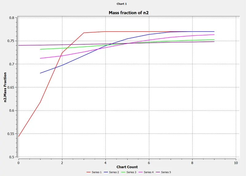
Lines are inserted using insert line command tof find the values at different locations.

Residual

Mass fraction of CH4

Plot of Mass fraction of CH4

Mass fraction of CO2

Plot

Mass fraction of H2O

Plot

Mass fraction of N2

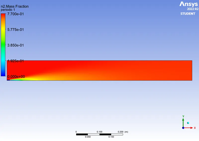
Plot

Mass fraction of O2

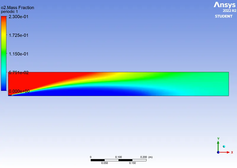
Plot

Mass fraction of NOX

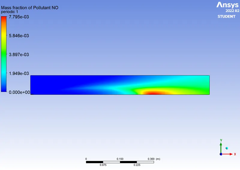
Plot

Mass fraction of SOOT

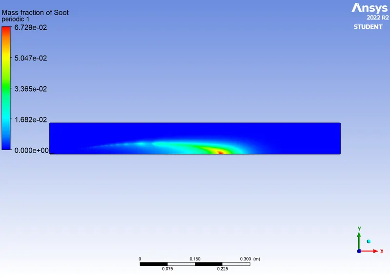
Plot

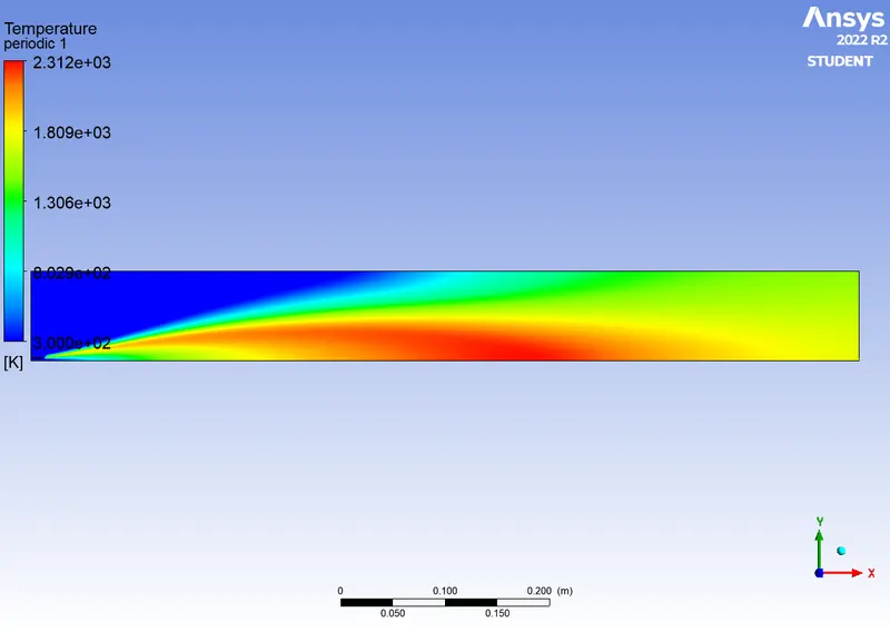
TEMPERATURE CONTOUR

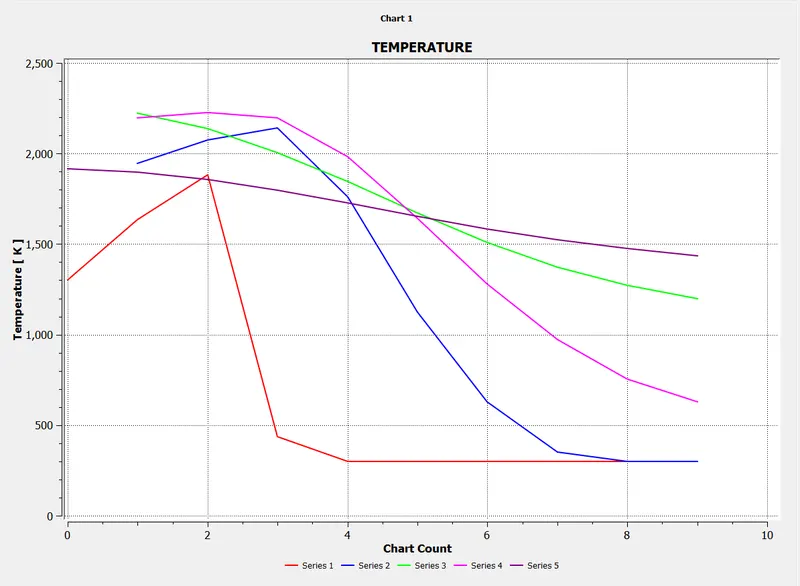
Plot

PART-2

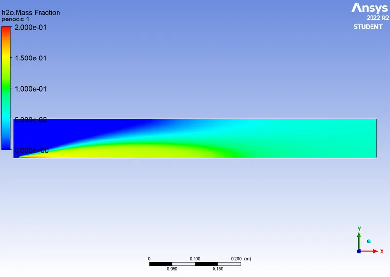
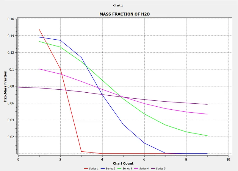
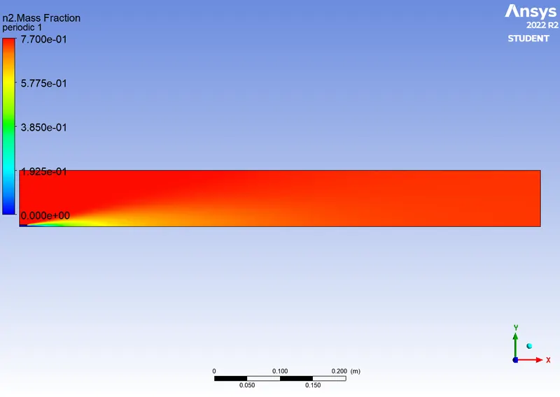
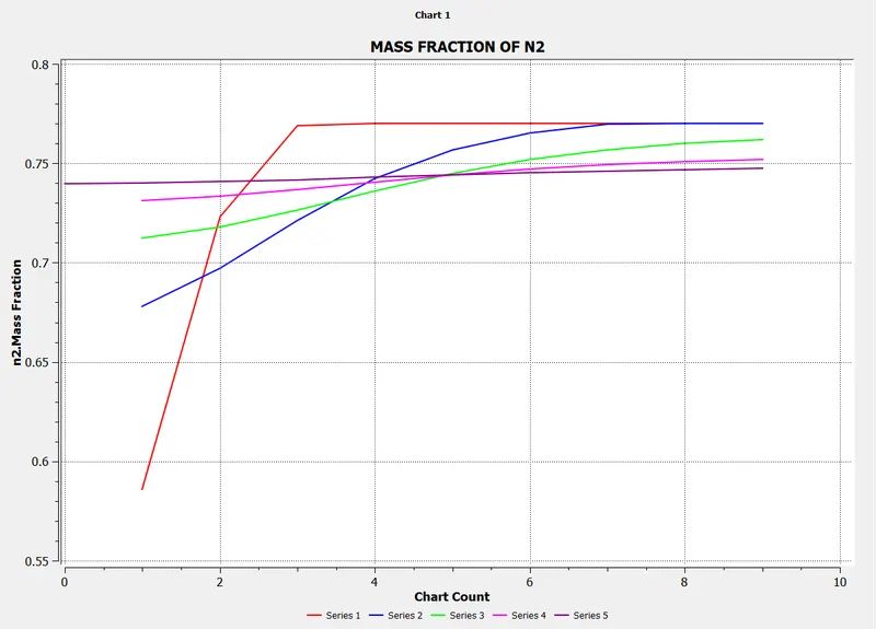
Addition of 20% water

Residual

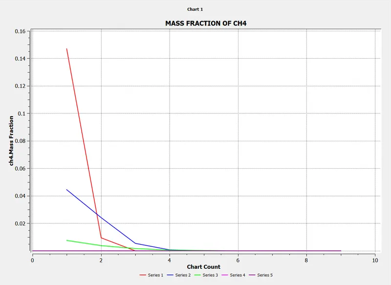
Mass fraction of CH4

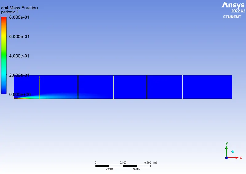
Plot

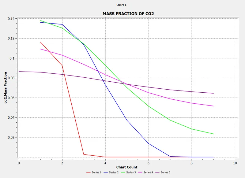
Mass fraction of CO2

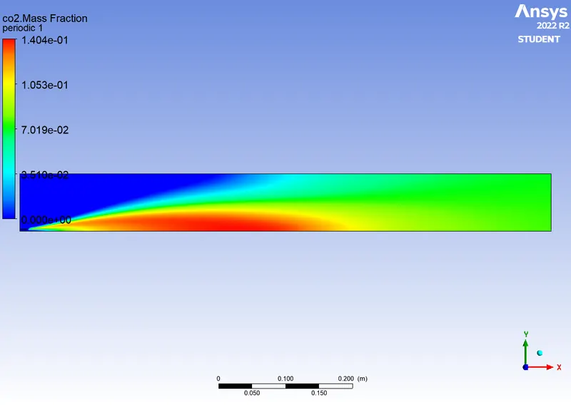
Plot

Mass fraction of H2O

Plot

Mass fraction of N2

Plot

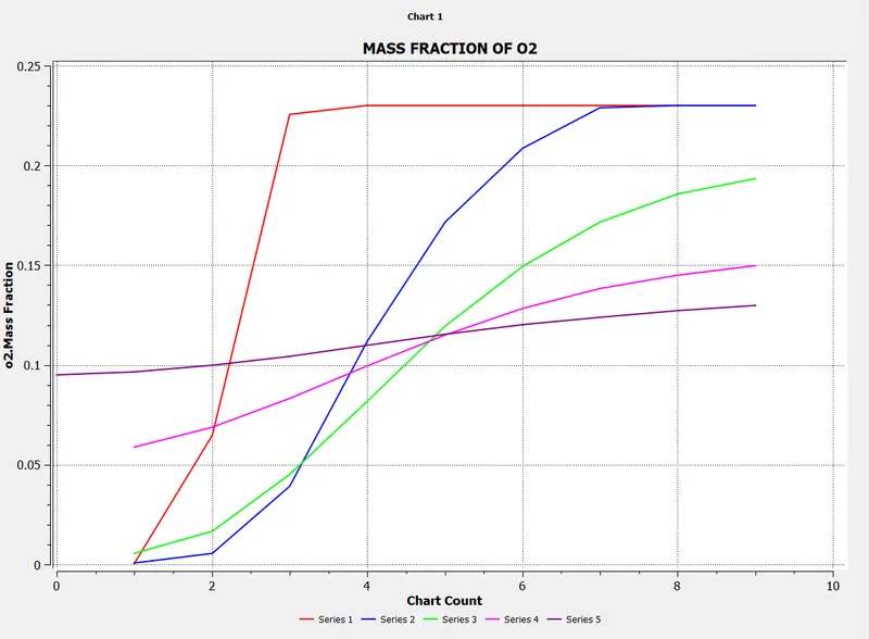
Mass fraction of O2

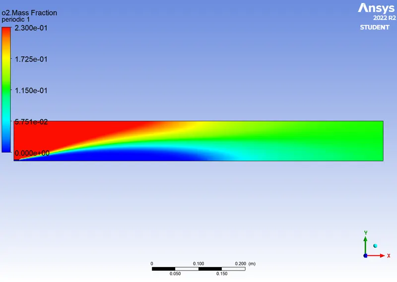
Plot

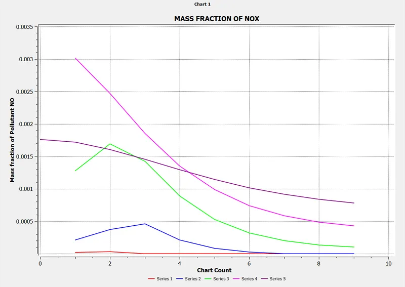
Mass fraction of NOX

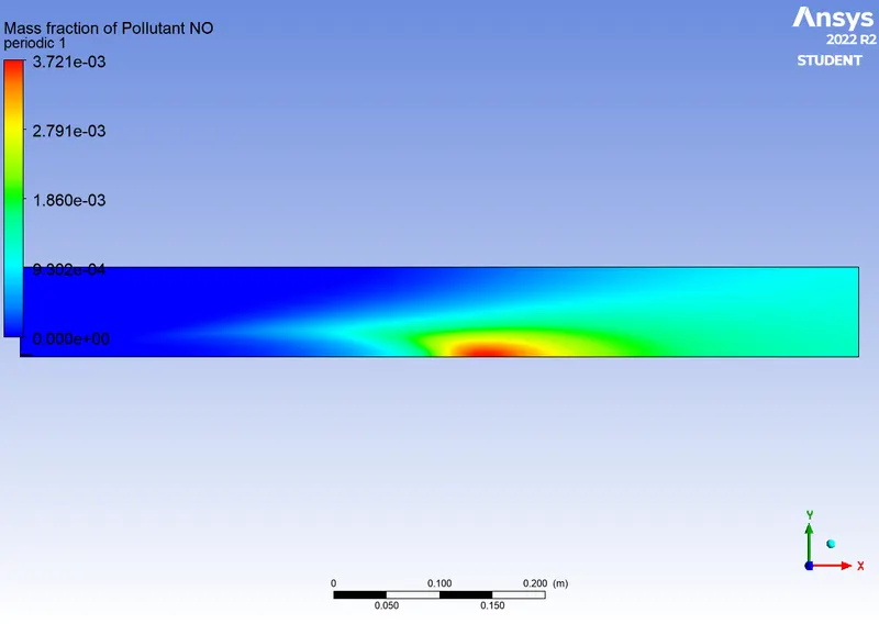
Plot

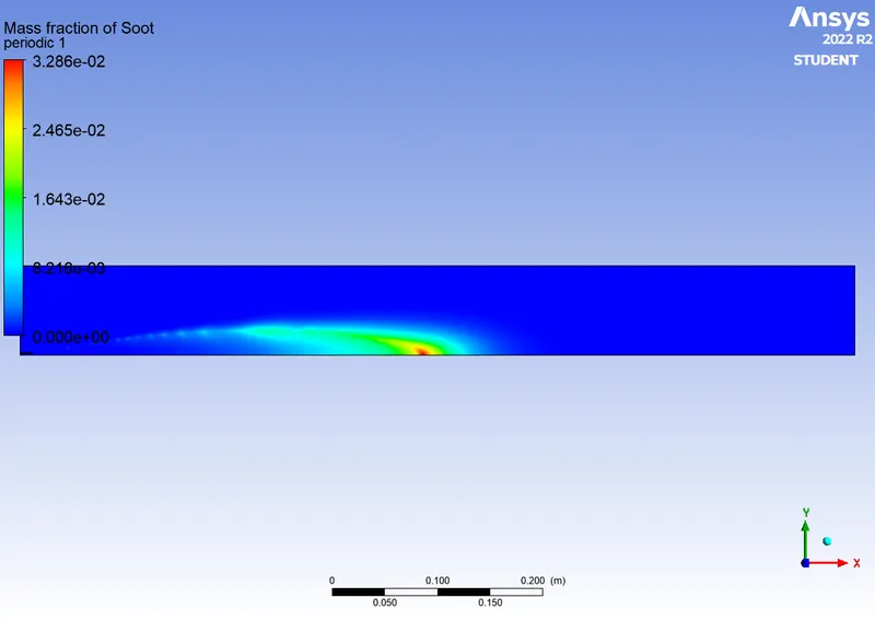
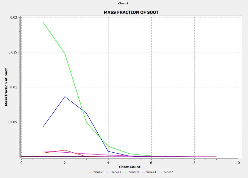
Mass fraction of SOOT

Plot

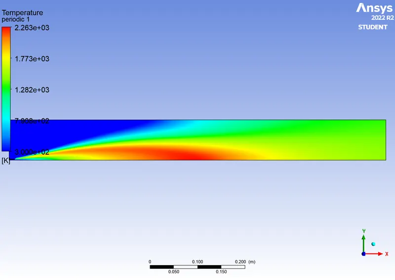
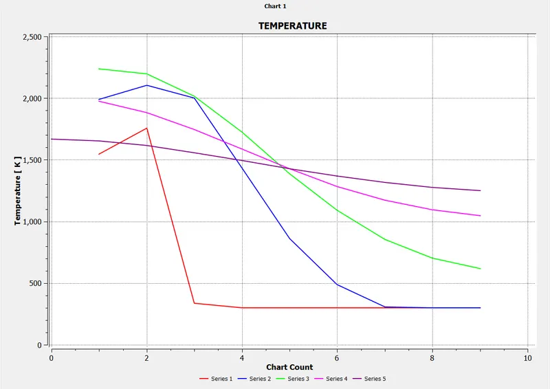
TEMPERATURE

Plot

Addition of 30% water

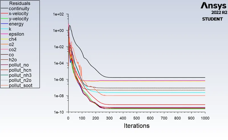
Residual

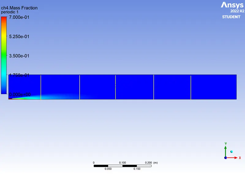
Mass fraction of Ch4

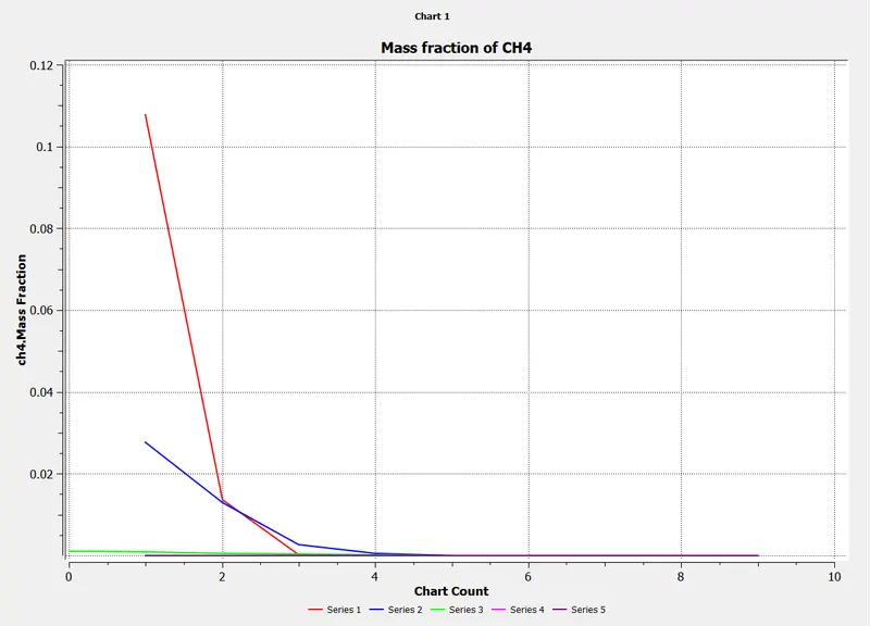
Plot

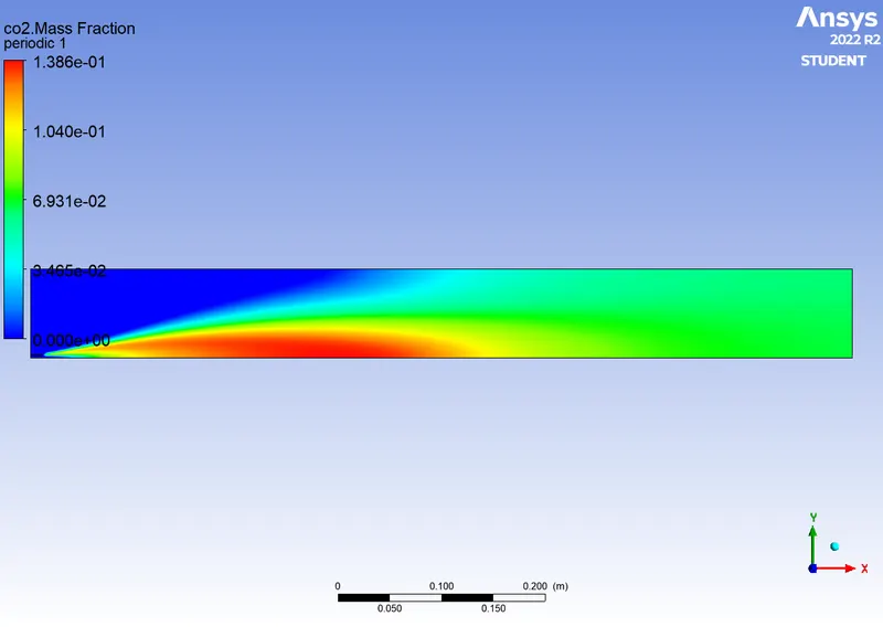
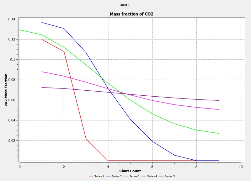
Mass fraction of CO2

Plot

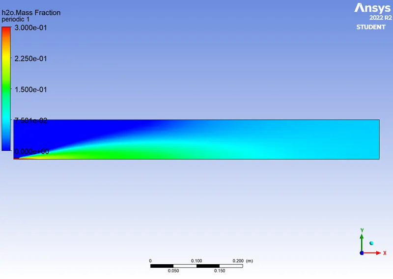
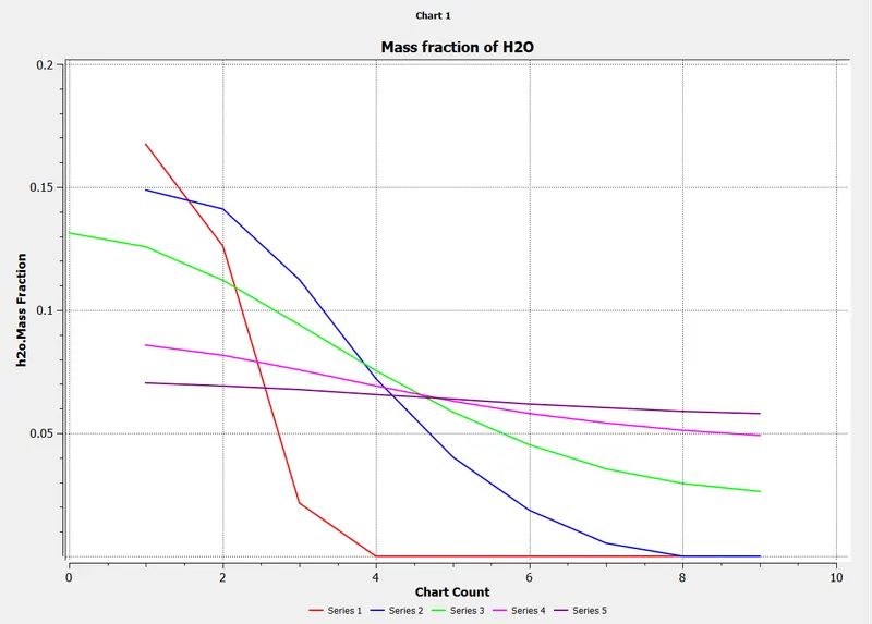
Mass fraction of H2O

Plot

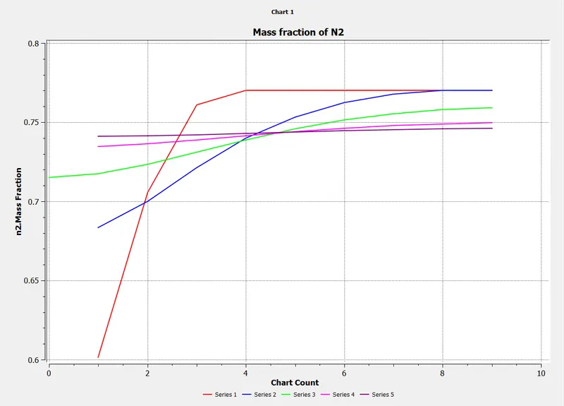
Mass fraction of N2

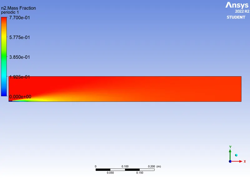
Plot

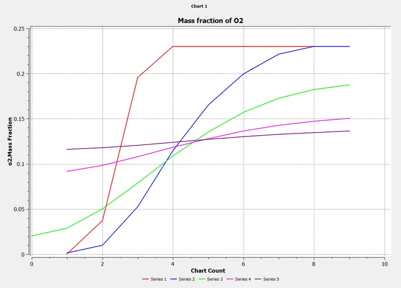
Mass fraction of O2

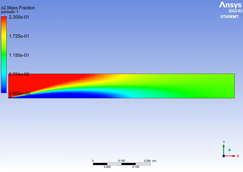
Plot

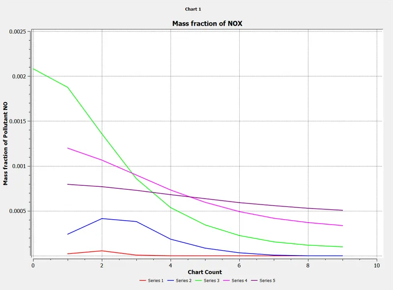
Mass fraction of NOX

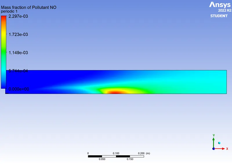
Plot

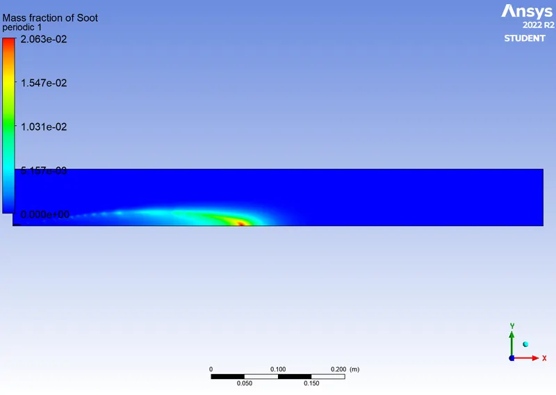
Mass fraction of SOOT

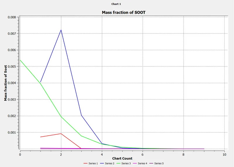
Plot

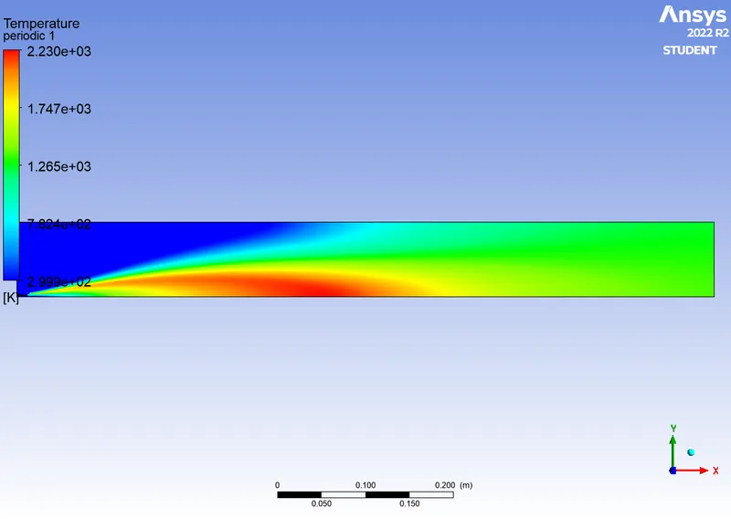
TEMPERATURE

Plot

Inference

Case	Water addition mass fraction	Temperature(k)	Mass fraction of NOX	Mass fractionn of SOOT
Part-1	0%	2.312	7.795e-3">7.795e−37.795e-3	6.729e-2">6.729e−26.729e-2
Part-2
case-1	20%	2.263	3.721e-3">3.721e−33.721e-3	3.286e-2">3.286e−23.286e-2
case-2	30%	2.230	2.297e-3">2.297e−32.297e-3	2.086e-2">2.086e−22.086e-2

Part-1(inference)

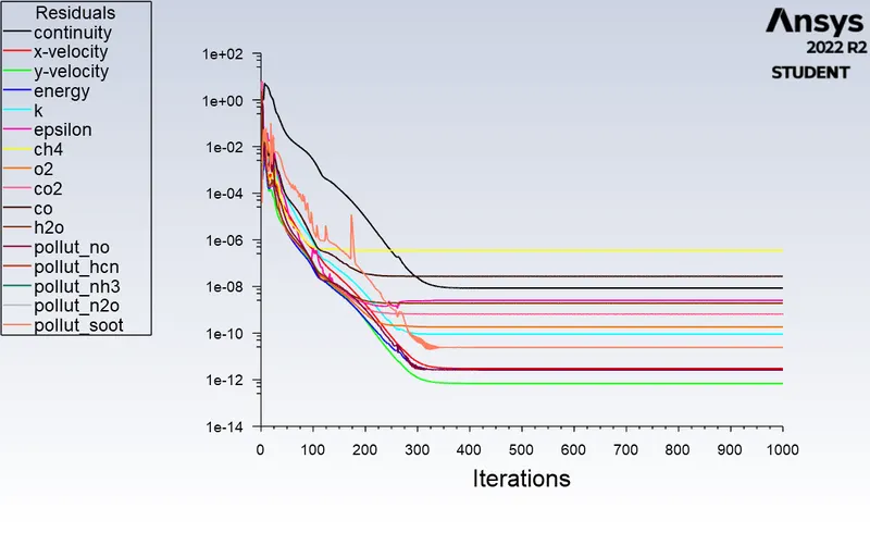
The solution converges at around 600 iterations.

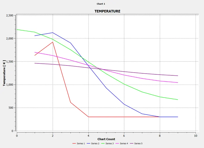
The temperature reaches the highest without water addition.

Part-2(Inference)

As the water content is increased the solution converges in lesser iterations.

Both the NOX and SOOT emissions gets reeduced with addition of water; higher the water fraction lesser the emmission.

The temperature reduces with the rise in water fraction.

CONCLUSION

The simulation provides a complete temperature distribution along the geometry. Contours of various species can be studied.
By adding water, the pollutant soot and NOx formation at the outlet is reduced. The plots of the same is also looked into.
Thus a combustion simulation on the combustor model has been done and the values are compared for different fractions water added.