Week 10 - Simulating Combustion of Natural Gas.
AIM:
To simulate the process of combustion on a model using a mixture of fuel and air and to plot the mass fraction probes at different intervals
To simulate the process for the combustion on a model using a mixture of fuel, air and different fractions of water from 5% to 30% and to plotthe mass fraction probes at diffrent line intervals for NOx, soot, Ch4, H20, CO2, O2, etc
DESCRIPTION:
Combustion is defined as a chemical reaction in which a hydrocarbon reacts wih an oxidant to form products, accompained by the release of energy in the form of heat
CHEMICAL KINETICS:
In general form, Fuel+air = Productos (global reaction) we say
But however, in reality global reaction is not the only reaction that is taking place. There are many elementary reactions and intermediatery reactions happening to form a global reaction which is all together called as Chemical kinetic.
So using a chemical kinetics solver means that we are solving all the equations for different intermediatary reactions , elementary reactions and different paths to predict the final product. This gives all the thermodynamic properties of the setup case.
This method depends on the path ways and also the time.
The importance of chemical kinetics is that the reaction pathways determine the following
- when combustion starts (ignition starts), if we are monitoring the data with time on x-axis and temperature on y-axis and the increase in temperature at particular time due to reactions happening and time associated with this is called Ignition delay.
- Heat release rate i.e can calculate the rate of work done
- Can compute the emissions i.e how much pollutants are produced.
When we are simulating combustion for a particular fuel we need to have the reaction mechanism which contains the elementary species and reactions. Without species a good result cannot be obtained.
For example low temperature combustion to simulate we need to have reactions that support the low temperature conditions in order to get the desired and acceptable results or else the simulation will be completely wrong along with the prediction.
The different types of elementary reaction types are
- Biomolecular reactions (most common): `A+BhArrC+D` reversible under some conditions
- Uni-molecular reactions, `AhArrB`(isomerization:same species having transformation of structure and `AhArrB+C` (decomposition: breaking into different parts line O2=O+O which combines with N and forms NO which is a pollutant).
- Termolecular reactions, `A+B+ChArrC+M` Here M is the third body species
Now after knowing the different types of elementary reactions and if we know how fast these reactions takes place than we can predict the reaction pathway.
In order to determine the pathway reaction we need
- Operating conditions like pressure and temperature
- Rate of reaction
DERIVATION FOR RATE OF REACTION FOR MULTISTEP MECHANISM
This case has 4 step reactions so its called multistep and in the reaction we have species viz H2, O2, HO2H, OH, HO2, O, M. So, we have 8 species and 4 reactions.
`H2+O2harr[[kf1],[kr1]]HO2+H` Here kf1 is the rate of forward reaction and kr1 is the rate of backward reaction
`H+O2harr[[kf2],[kr2]]OH+O`
`OH+H2harr[[kf3],[kr3]]H2O+H`
`H+O2+Mharr[[kf4],[kr4]]HO2+M`
On solving the above equations we get the ODE with concentrations for each speciesFor
For O2
`(d[o2])/(dt)=kr1[HO2][O2]-kf1[H2][O2]+kr2[O][OH]-kf2[H][O2]+kr4[M][HO2]-kf4[H][O2][M]`
For H
`(d[H])/(dt)=kf1[H2][O2]-kr1[HO2][H]+kr2[OH][O]-kf2[H][O2]+kf3[OH][H2]-kr3[H][H2O]+kr4[M][HO2}-kf4[H][O2][M]`
For H2
`(d[H2])/(dt)=kr1[HO2][H]-kf1[H2][O2]`
For H2O
`(d[H2O])/(dt)=kf3[OH][H2]-kr3[H][H2O]`
For HO2
`(d[HO2])/(dt)=kf1[H2][O2]-kr1[HO2][H]+kf4[H][O2][M]-kr4[M][HO2]`
For O
`(d[O])/(dt)=kf2[H][O2]-kr2[OH][O]`
For OH
`(d[OH])/(dt)=kf2[H][O2]-kr2[OH][O]+kr3[H][H2O]-kf3[OH][H2]`
So we have 7 coupled ODEs with -ve for the one whose concentration is decreasing and + for ones whose concentration is not decreasing. Solving these all we get the pollutants but it takes a lot of time so we use CFD to solve them.
We use here the compact notations as follows
| j | SPECIES |
| 1 | O2 |
| 2 | H2 |
| 3 | H2O |
| 4 | HO2 |
| 5 | O |
| 6 | H |
| 7 | OH |
| 8 | M |
| i | REACTION |
| 1 | R1 |
| 2 | R2 |
| 3 | R3 |
| 4 | R4 |
For the reactants side we make a matrix with columns containing the number of species and rows containing the number of reactions as follows
`Vj^' = [[1,1,0,0,0,0,0,0],[1,0,0,0,0,1,0,0],[0,1,0,0,0,0,1,0],[1,0,0,0,0,1,0,1]]`
And for products
`Vj^('')=[[0,0,0,1,0,1,0,0],[0,0,0,0,1,0,1,0],[0,0,1,0,0,1,0,0],[0,0,0,1,0,0,0,1]]`
POSSIBLE TYPES OF COMBUSTION SIMULATION:
Based on mixing
- Non-premixed combustion (direct injection, late injection): In this, fuel and oxidizer enter the reaction zone in distinct streams.It occurs during direct injection or late injection of fuel in IC engines.For example are pulvarized coal furnaces, diesel internal combustion engines and pool fires.
- Premixed combustion (carburetor): In this, fuel and oxidizer are mixed at molecular level prior to ignition.Combustion occurs as flames propagating into the unburnt reactants. Examples are aspirated internal combustion engines, gas-leak explosions.
- Partially premixed: In this premixed flames with non-uniform fuel-oxidizer mixtures of equivalence ratios. For exaple jets discharging into an inert atmosphere.
Based on phase
- Fluid phase (volumetric reactions): combustion takes place in the fluid region.
- Wall (surface reactions): Cpmbustion takes place on the wall or a solid surface
- Particles (surface reaction):Combustion takes place on the lagrangian particles.Combustion of coal is an example f particle combustion.
- Porous region:Combustion takes place in porous region.The reaction in an after treatment system is an example.
COMBUSTION SOURCE CALCULATION
1.Finite rate chemistry:Accurate but slow
2.Mixing based models: The eddy dissipation model and its fast but requires user experience
3.Finite rate eddy dissipation model: Combustion of both finite rate chemistry and eddy dissipation model and is used to prevent instantaneous buring (mixeed is burnt problem).
COMBUSTION REACTIONS:
The general reaction of combustion is given as `CH4+ar(O2+3.76N2)->aCO2 + bH2O + cN2`
Balancing the above equation for C,H2,O2,N2 we get
a=1
b=2
ar=a+b/2
c=15.04
The above values corresponds to the number of moles of the given species
Fuel: 1 mole of CH4
Air: 2 moles of O2+7.52 moles of N2
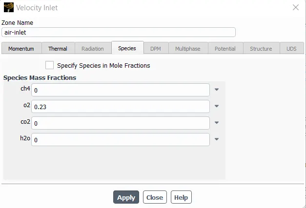
Therefore, The mole fraction of O2 = 2/(2+7.52) = 0.21
and mole fraction for N2 = 7.52/(2+7.52) = 0.79
The mass fraction for O2=`(0.21*16)/((0.21*16)+(0.79*14))`=0.23
for N2= `(0.79*16)/((0.21*16)+(0.79*14))`=0.77
PROCEDURE FOR SIMULATION:
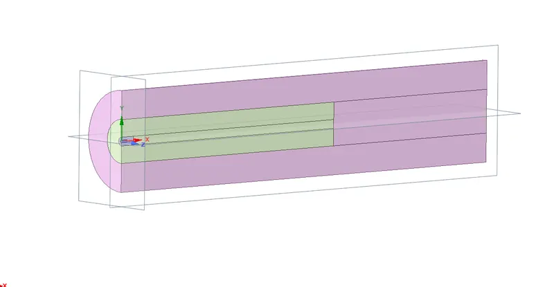
As solver takes a lot of time for simulation it takes a lot of time so in spaceclaim we import the geometry and create the planes and cut it in z-direction.
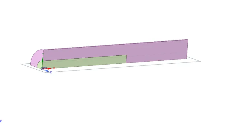
Then again we create the plan in x-direction and cut along the plane
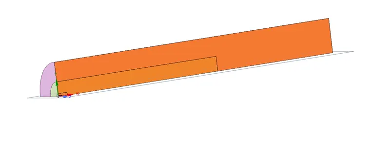
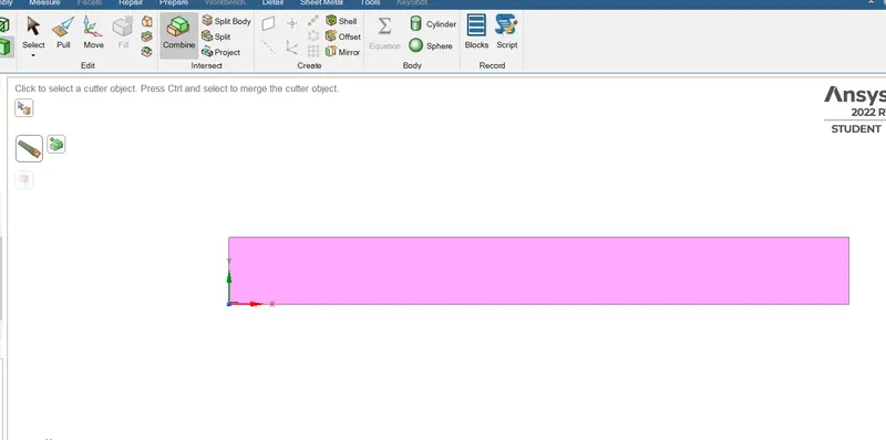
Then we select the faces and paste in to new design window to get the 2D model
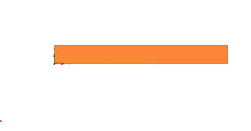
After pasting it in 2D model we get the following
MESHING
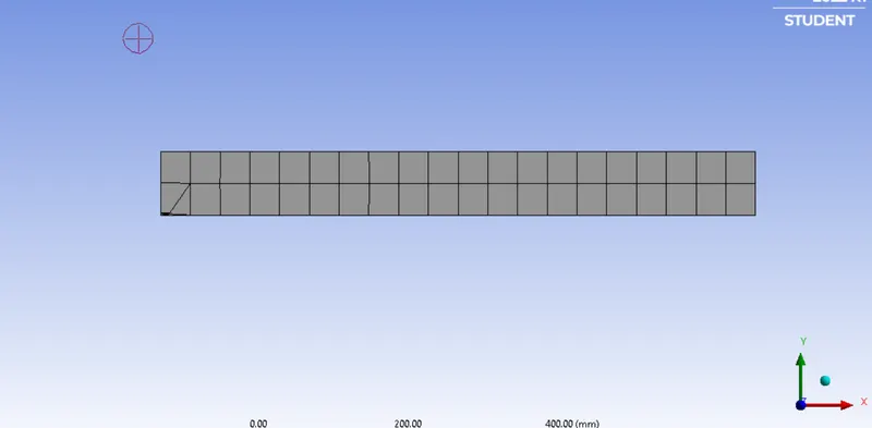
The default mesh looks as follows
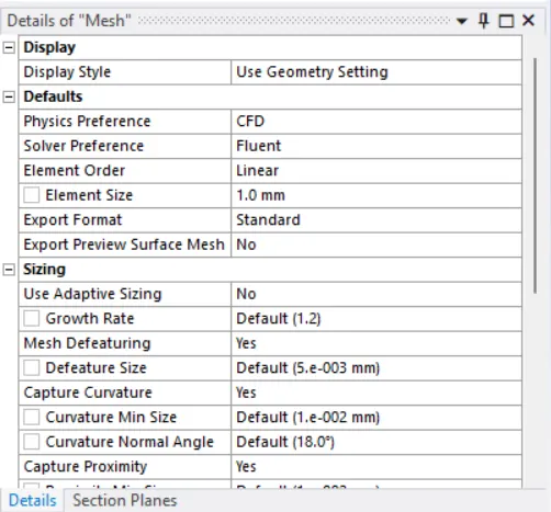
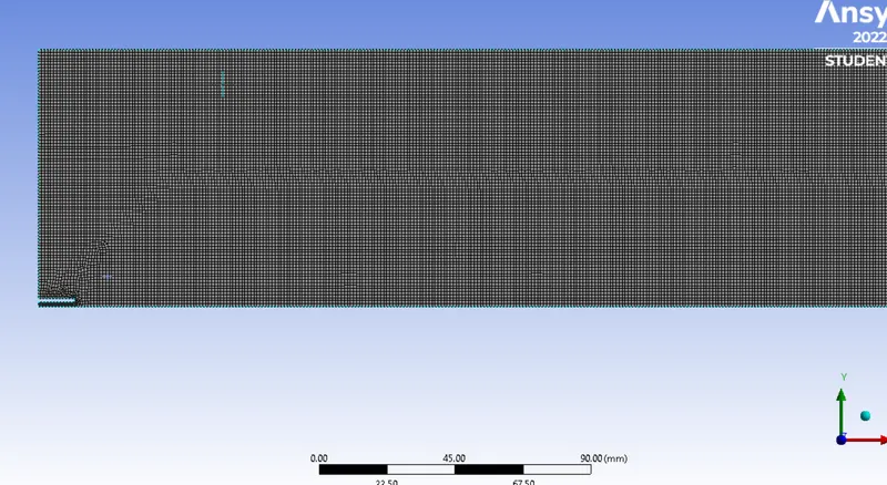
Making the mesh finer with 1mm element size with proximity capture YES
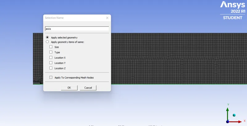
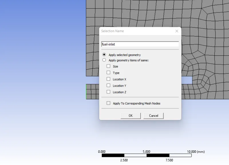
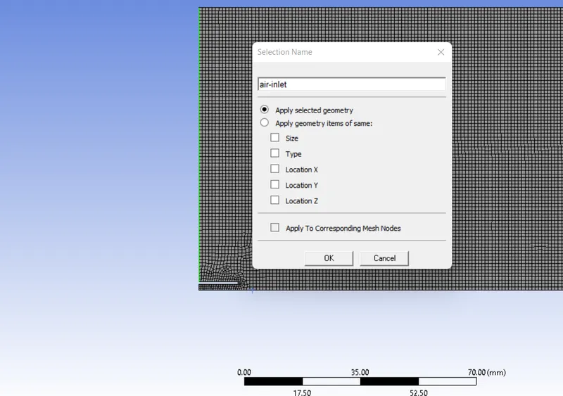
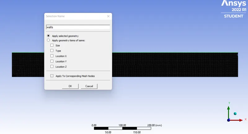
Now naming the parts,
For axis along x direction
For fuel inlet
For air inlet
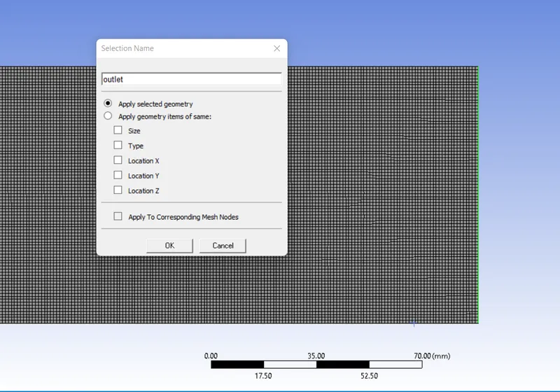
For walls
For outlet
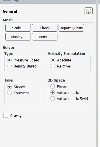
ANSYS FLUENT
We need to select the pressure based steady state axisymmetric solver
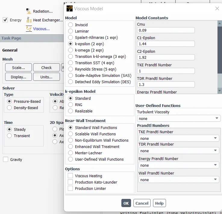
Enabling the energy equation and choosing the k-epsilon method to get the eddy dissipation model
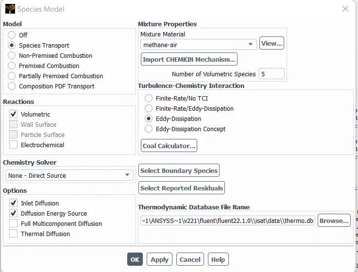
Then for species model enable the species tranport, volumetric with inlet diffusion and diffusion energy source with methane-air material with eddy dissipation
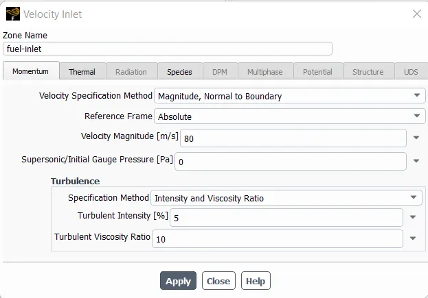
For boundary conditions
For inlet
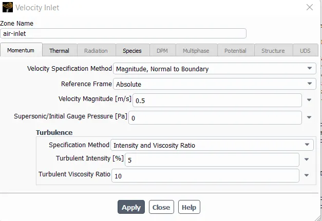
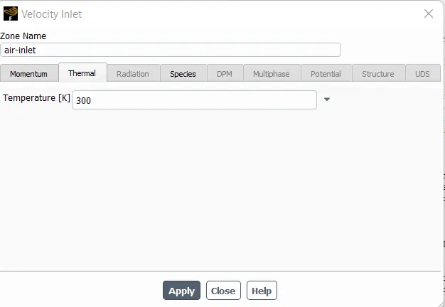
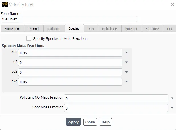
For inlet mass fractions
For fuel inlet
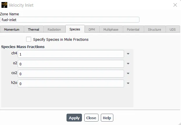
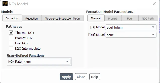
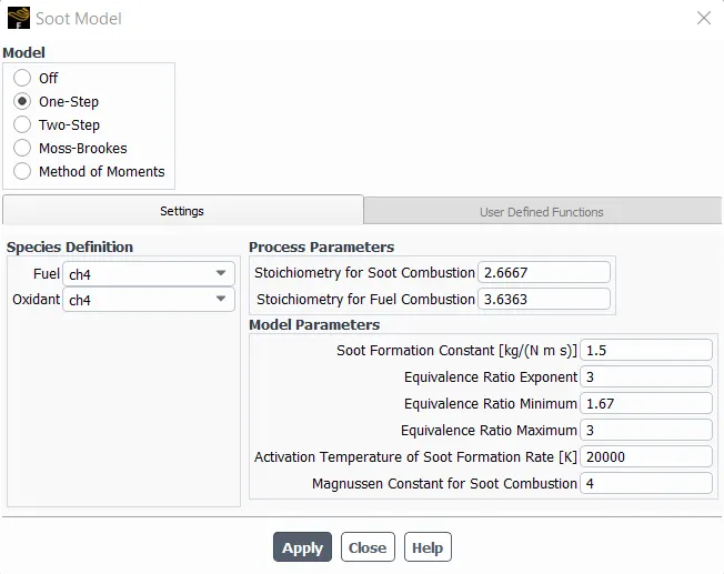
For outlet we use pressure outlet and for walls the wall boundary conditions
Here as we have air and fuel they burn through ignition source but here as we are using the eddy dissipation model the fuel fuel burning rate is not governed by the energy source but is governed by the turbulence.
Solving with hybrid initialization
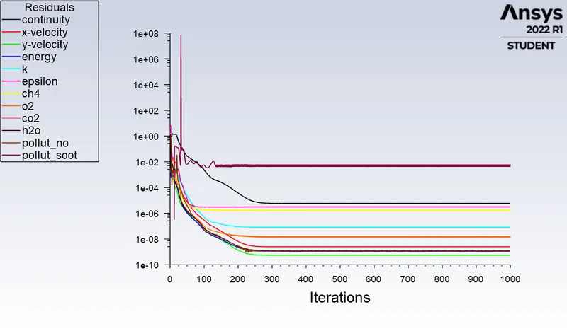
Running simulation for 1000iterations
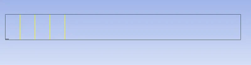
Creating the line probes post processing of CFD
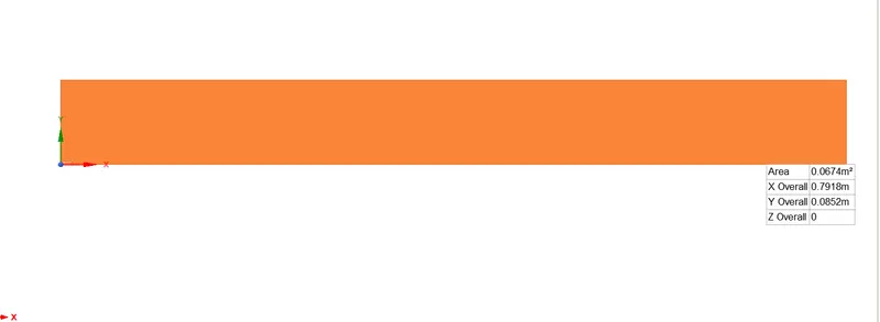
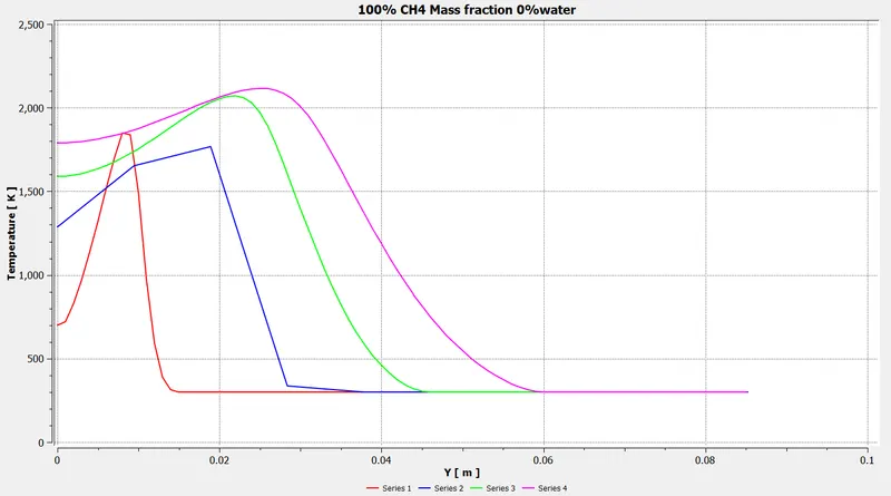
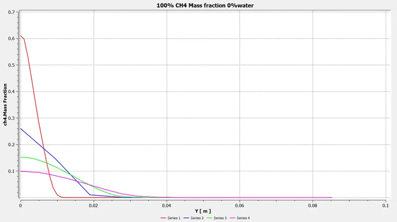
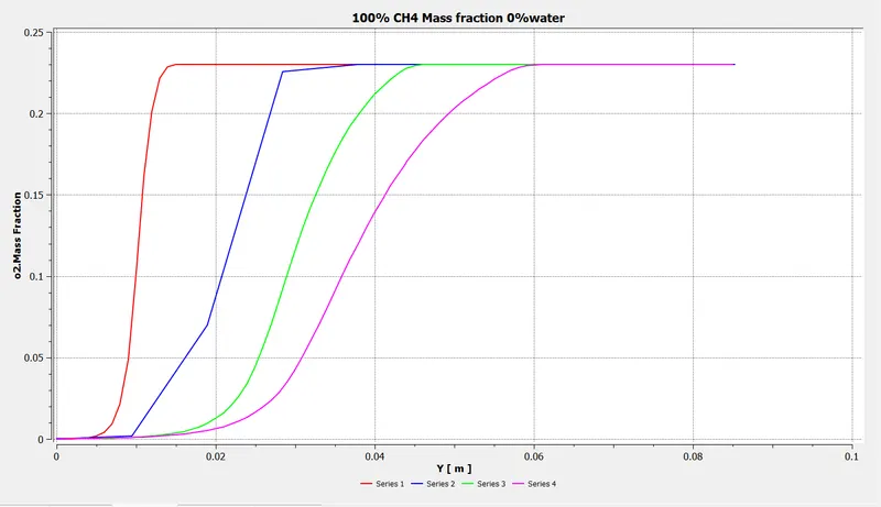
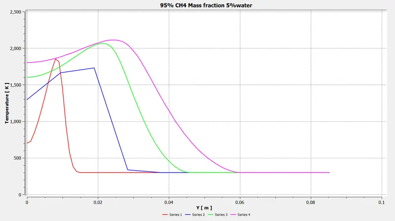
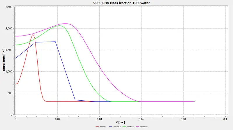
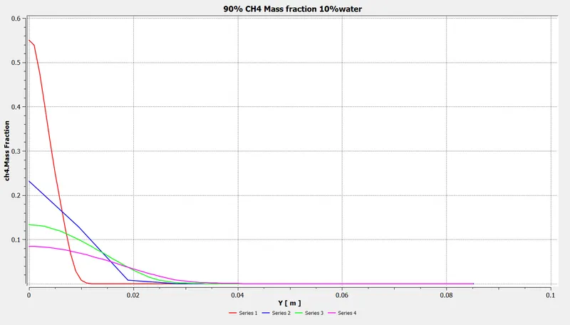
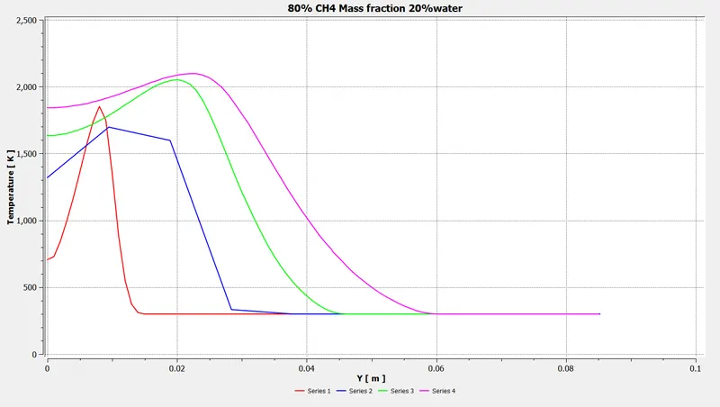
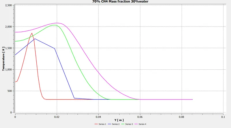
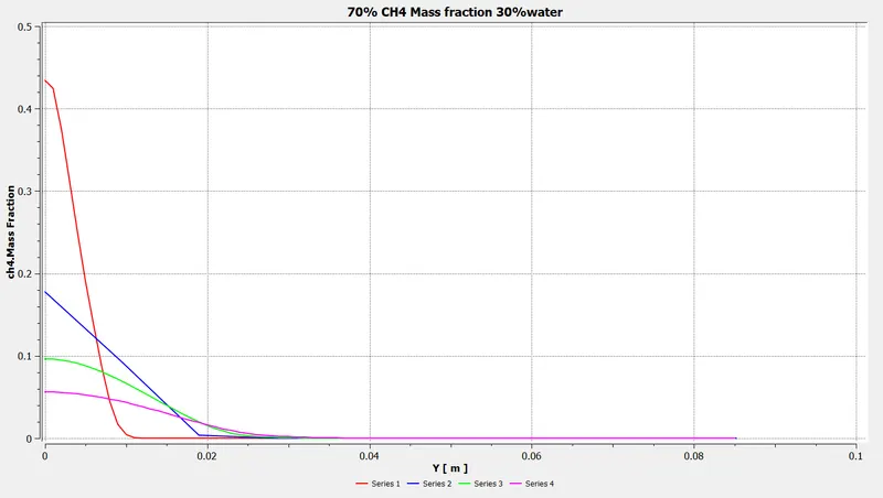
Line 1 (0.05,0,0)(0.05,0.0852,0)
Line 2 (0.1,0,0)(0.1,0.0852,0)
Line 3 (0.15,0,0)(0.15,0.0852,0)
Line 4 (0.2,0,0)(0.2,0.0852,0)
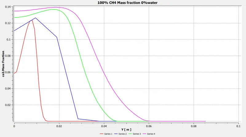
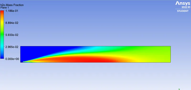
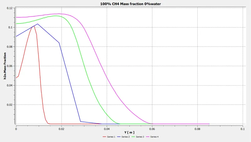
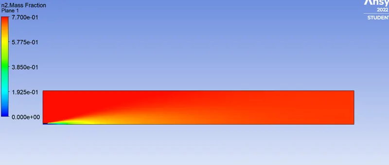
CASE-I:SIMULATION FOR COMBUSTION MODEL WITH 100% CH4 AND 0% H20 MASS FRACTION:
The residuals are
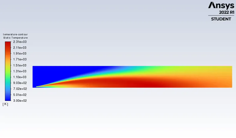
The temperature contours are
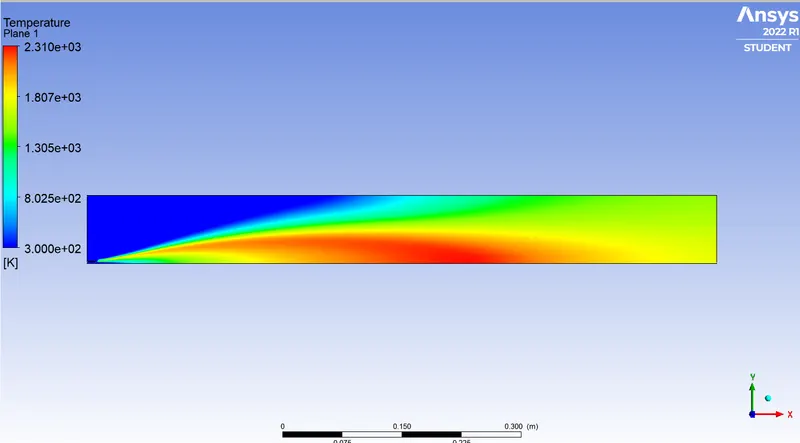
The temperature plane is
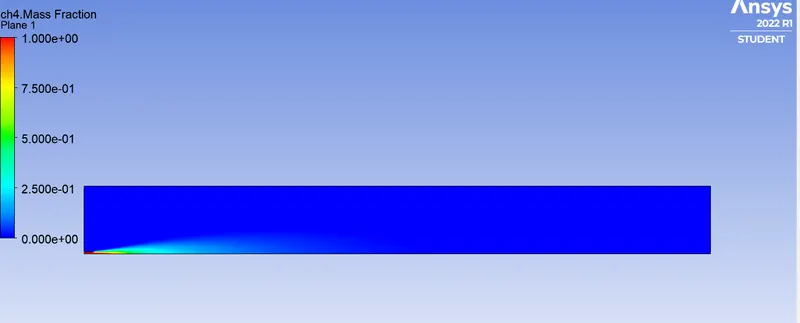
The CH4 mass fraction
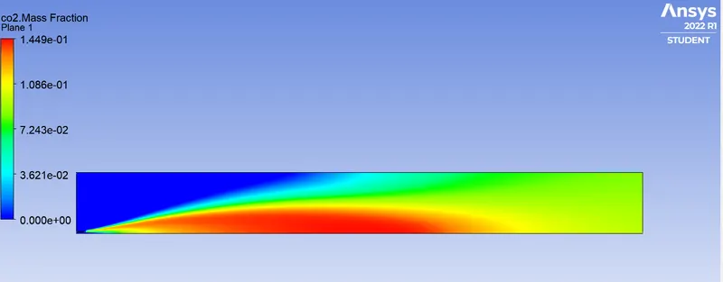
The CO2 mass fraction
The H2O mass fraction
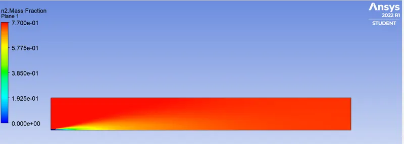
The N2 mass fraction
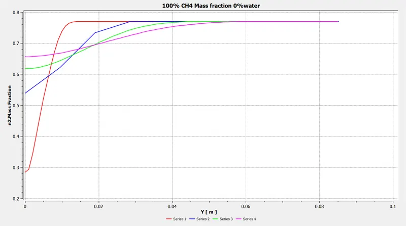
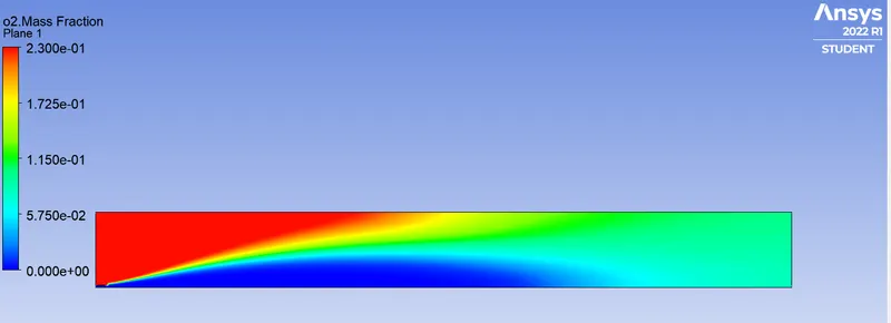
The O2 mass fraction
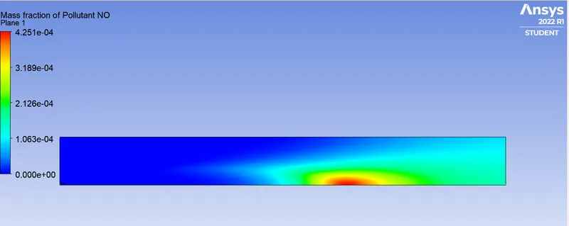
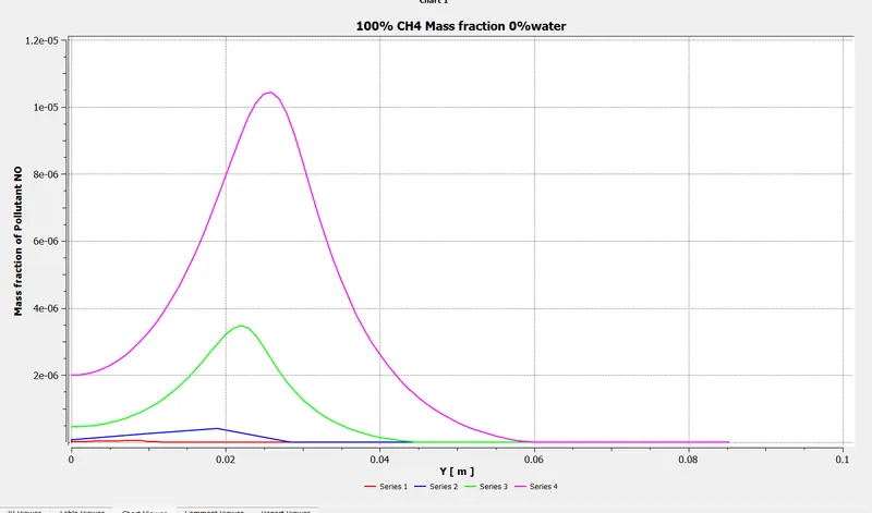
The pollutant NO mass fraction
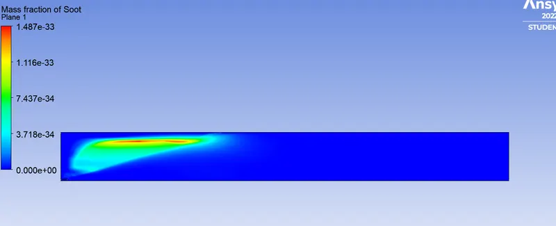
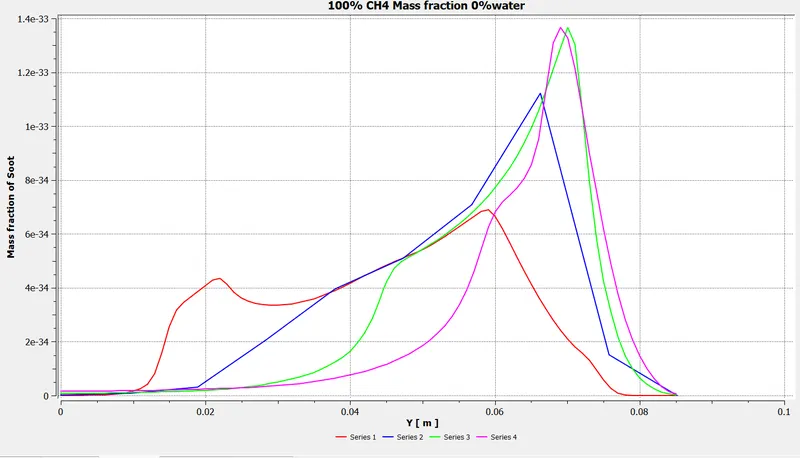
The soot mass fraction
CASE-II: SIMULATION FOR COMBUSTION MODEL WITH 95% CH4 AND 5% H20 MASS FRACTION
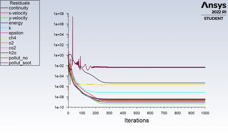
The residuals are
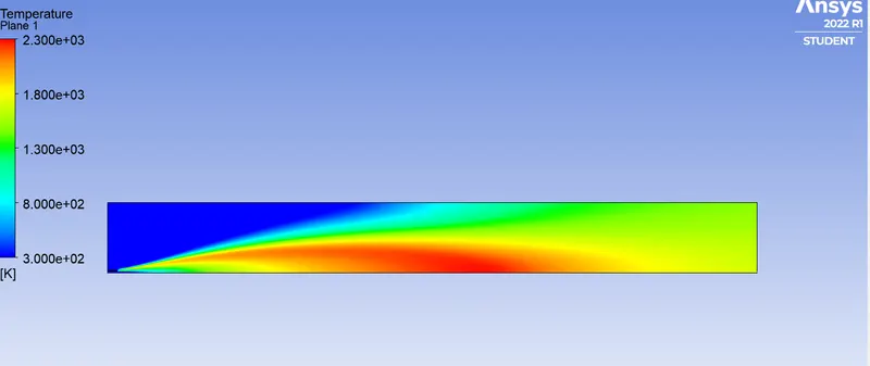
The temperatures are
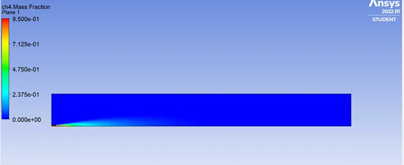
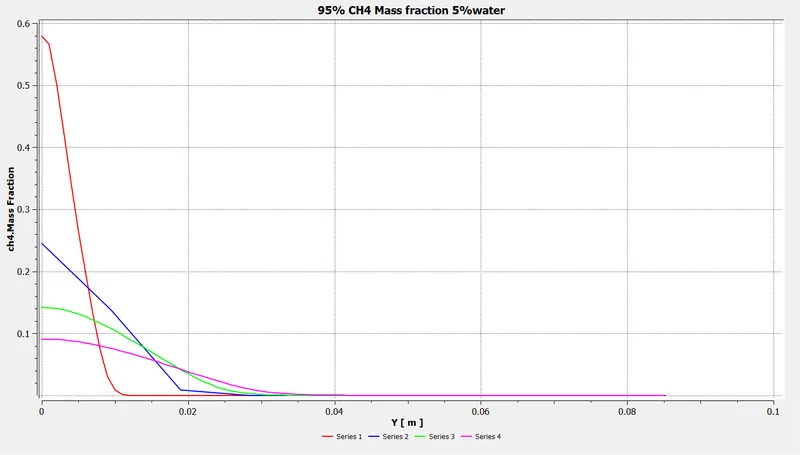
The CH4 mass fraction is
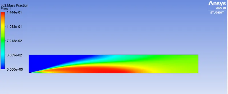
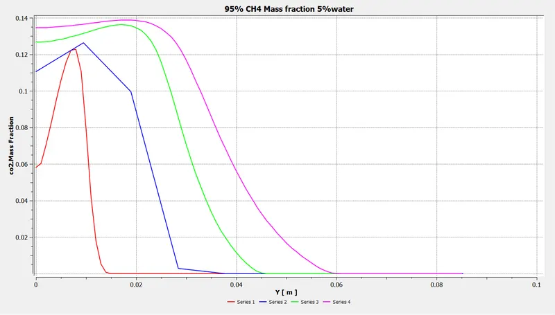
The CO2 mass fraction is
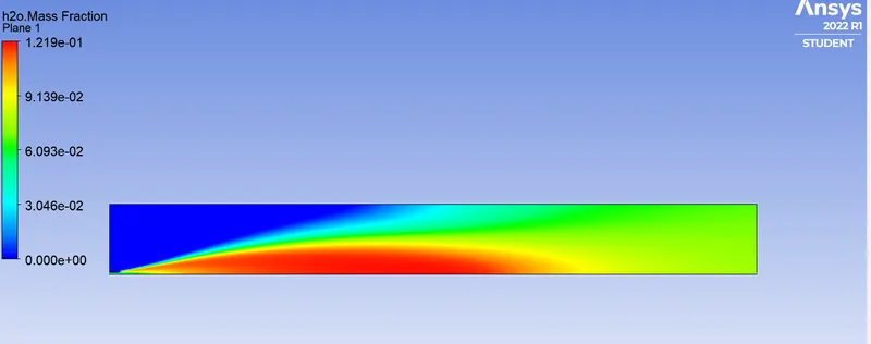
The H2O mass fraction is
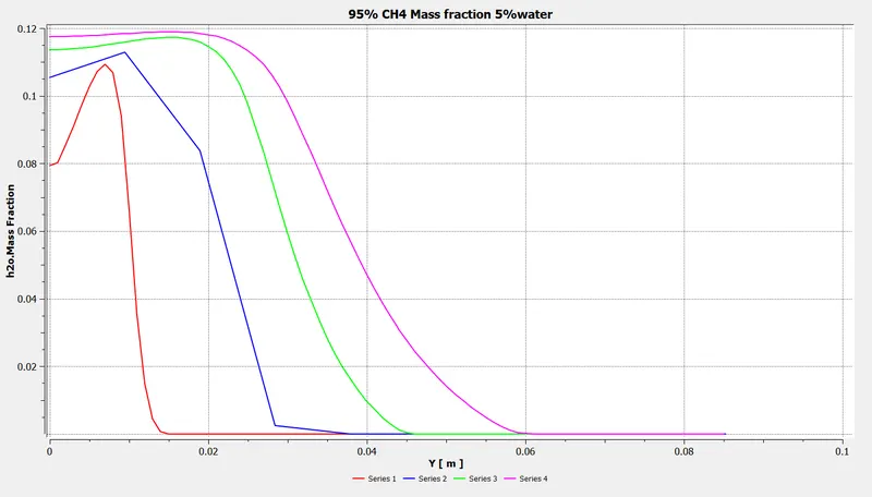
The N2 mass fraction is
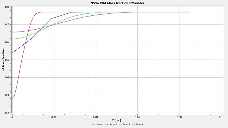
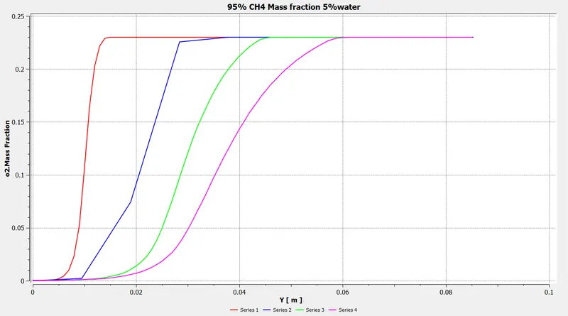
The O2 mass fraction is
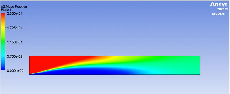
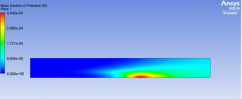
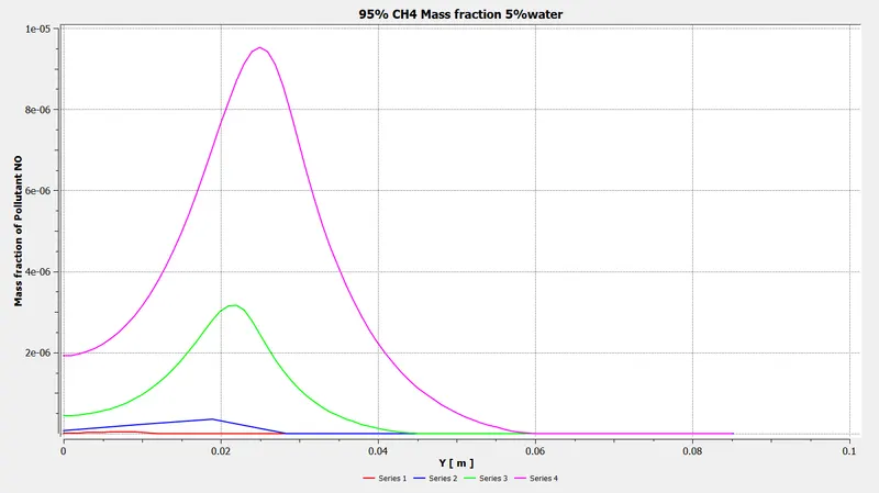
The Pollutant NO mass fraction is
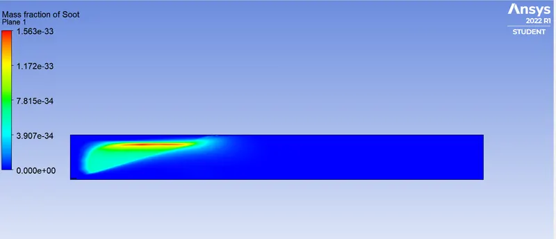
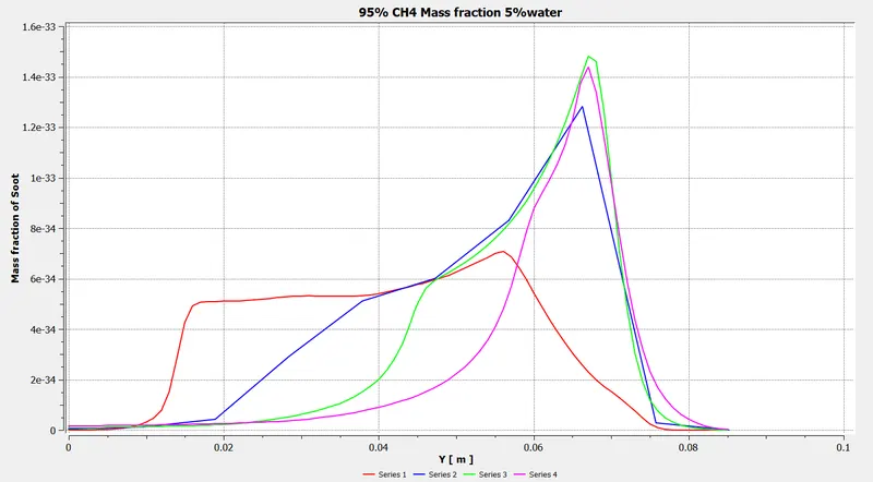
The soot mass fraction is
CASE-III:SIMULATION FOR COMBUSTION MODEL WITH 90% CH4 AND 10% H20 MASS FRACTION
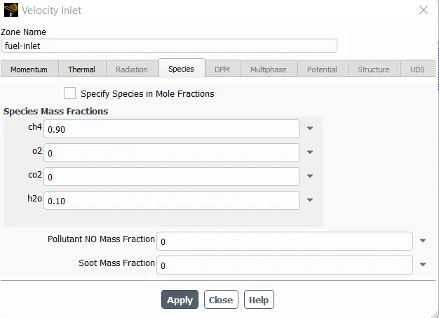
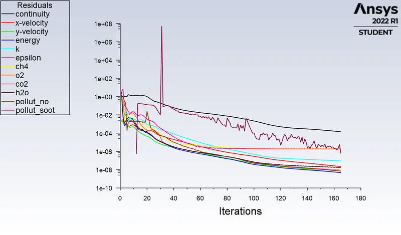
The residuals are
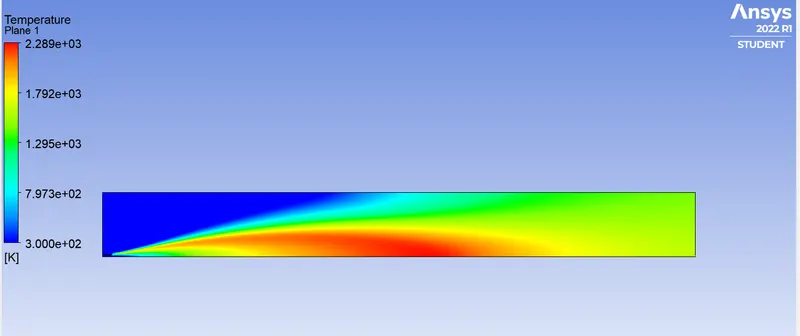
The temperature plane is
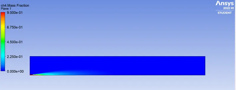
The CH4 mass fraction is
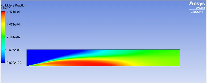
The CO2 mass fraction is
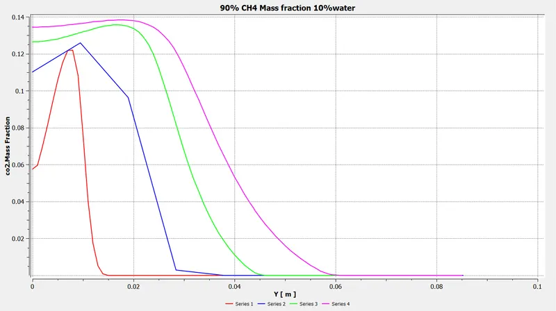
The H2O mass fraction is
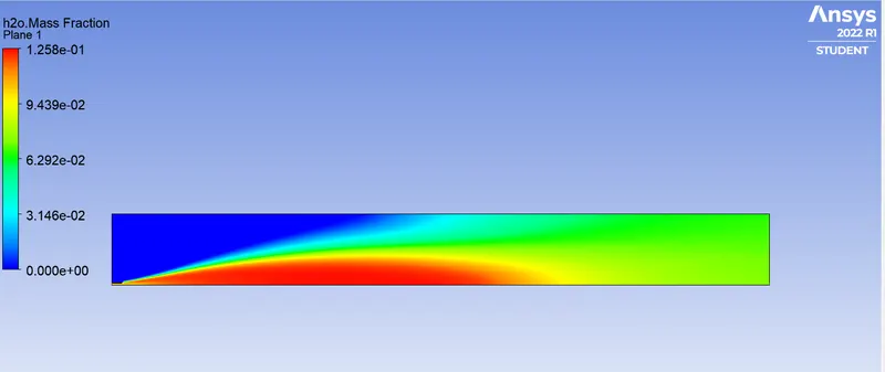
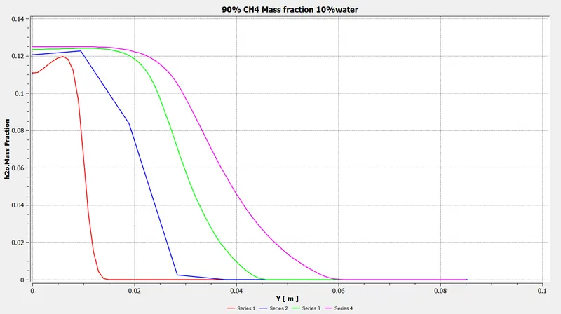
The N2 mass fraction is
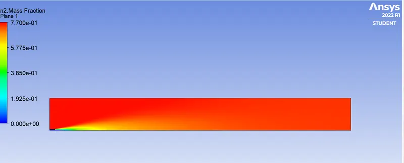
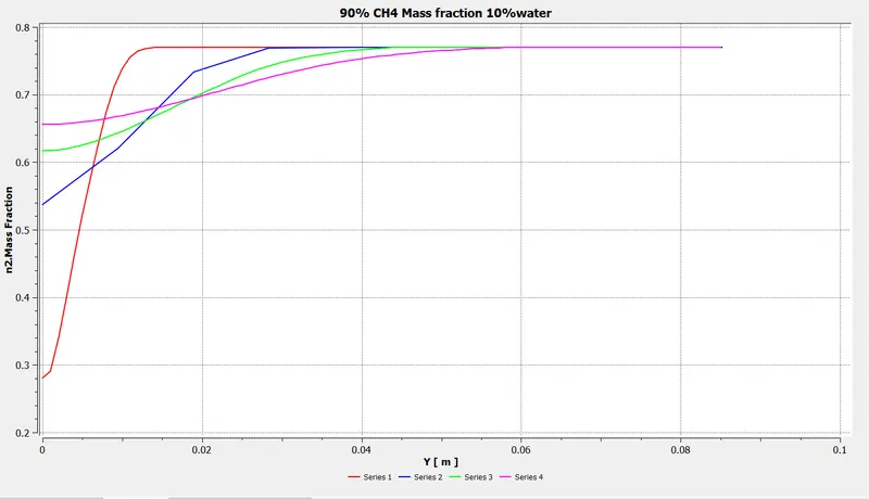
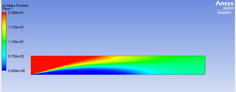
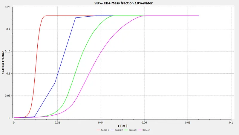
The O2 mass fraction is
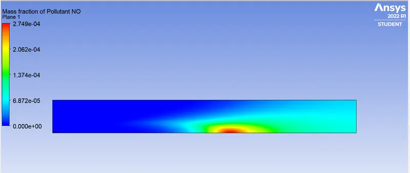
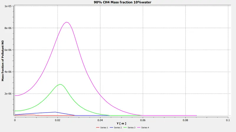
The pollutant NO mass fraction is
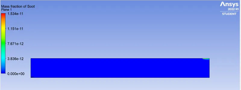
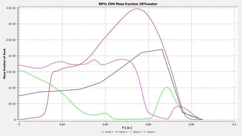
The soot mass fraction is
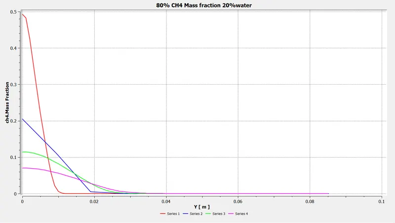
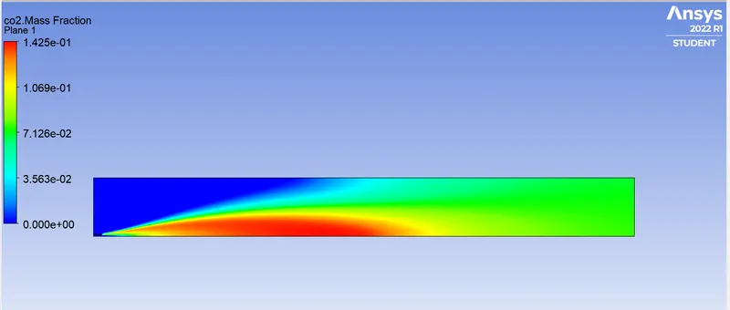
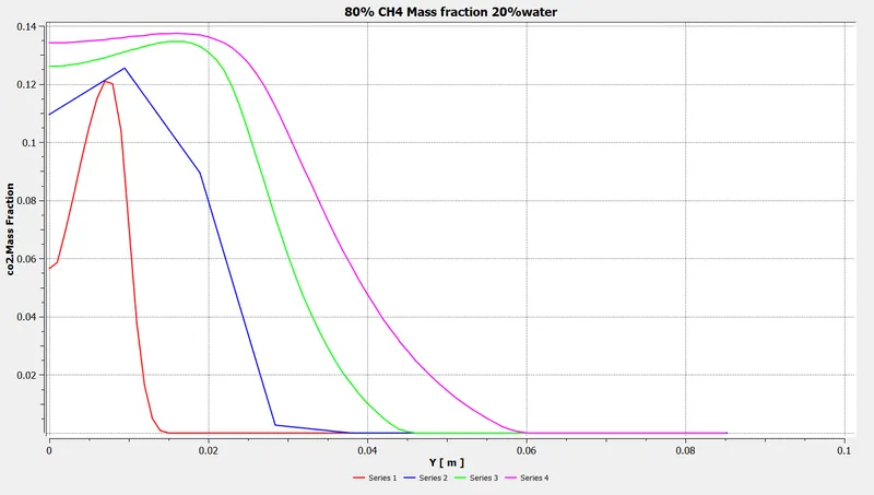
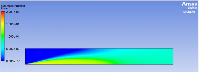
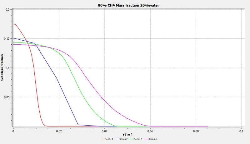
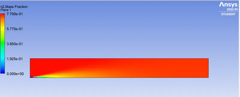
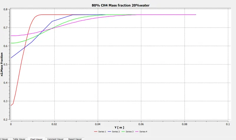
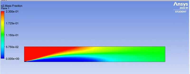
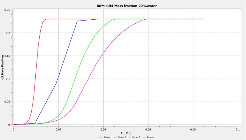
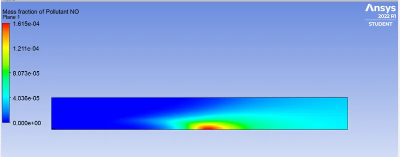
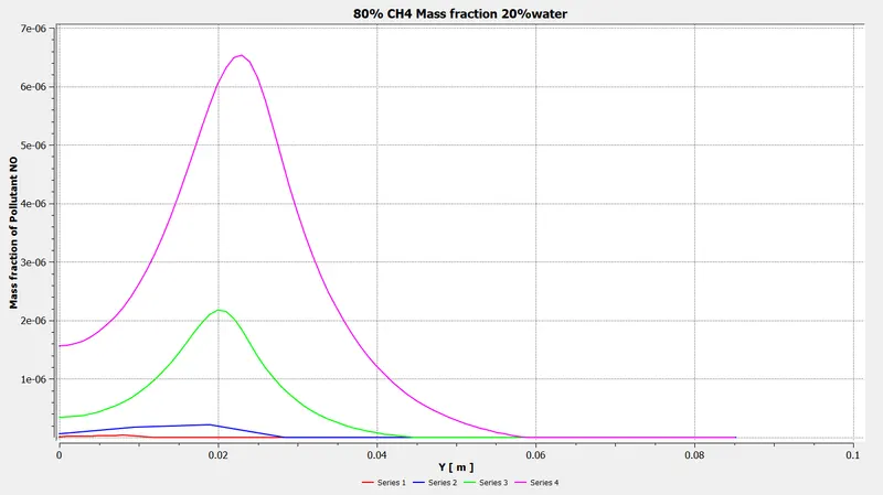
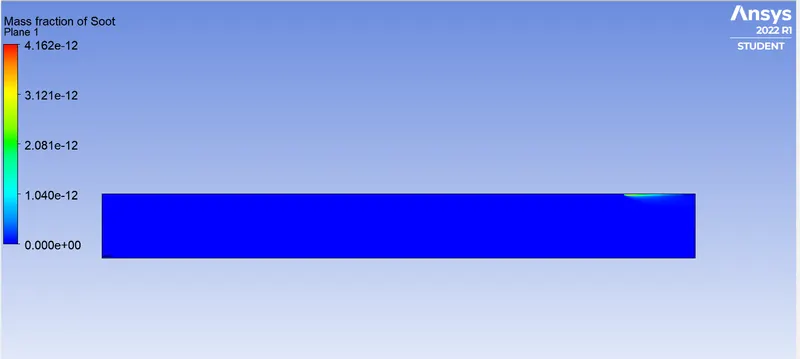
CASE-IV:SIMULATION FOR COMBUSTION MODEL WITH 80% CH4 AND 20% H20 MASS FRACTION
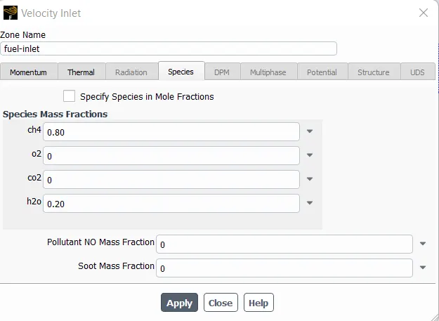
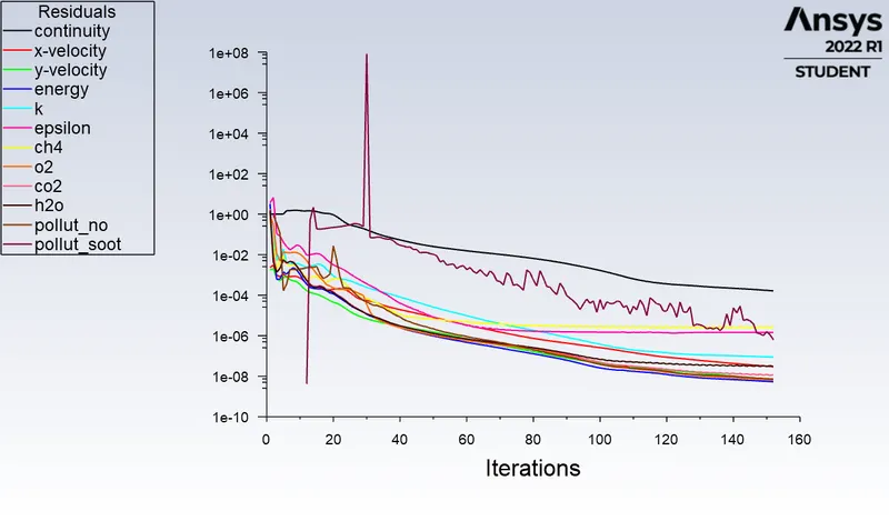
The residuals are
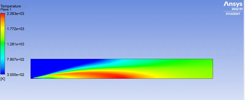
The temperature plane is
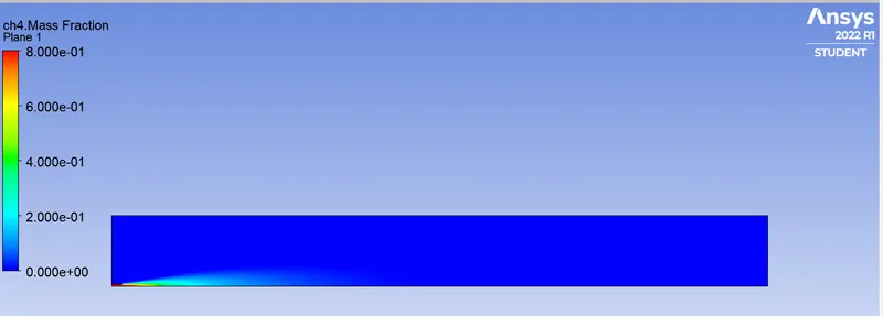
The CH4 mass fraction is
The CO2 mass fraction is
The H2O mass fraction is
The N2 mass fraction is
The O2 mass fraction is
The pollutant No mass fraction is
The soot mass fraction is
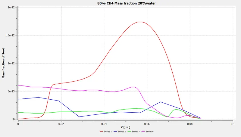
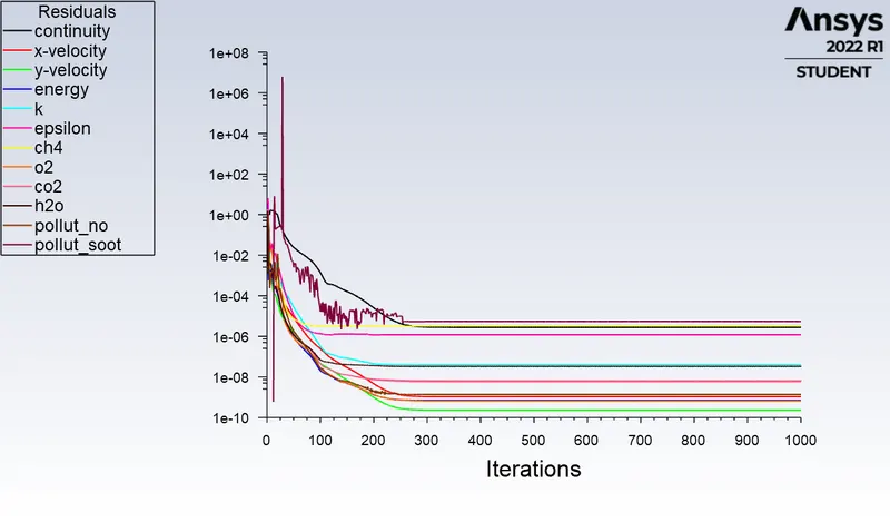
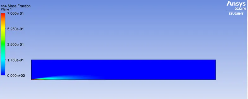
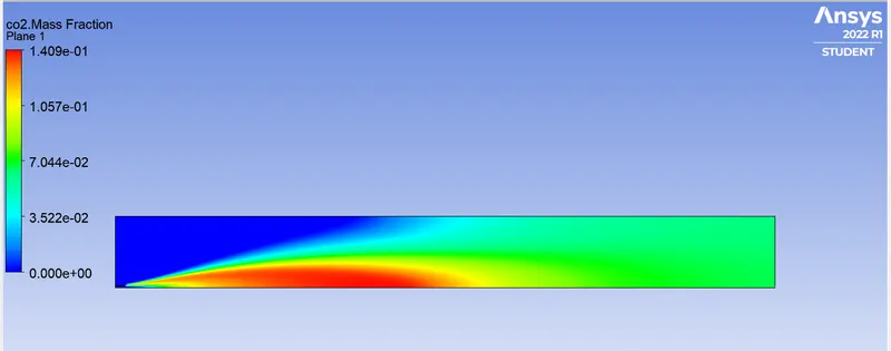
CASE-V:SIMULATION FOR COMBUSTION MODEL WITH 70% CH4 AND 30% H20 MASS FRACTION
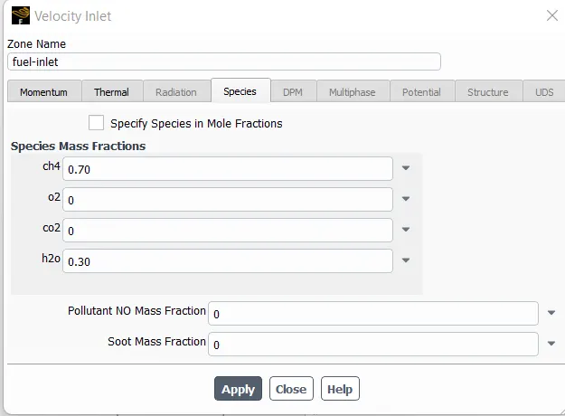
The residuals are
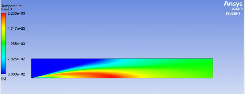
The temperature plane is
The CH4 mass fraction is
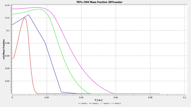
The CO2 mass fraction is
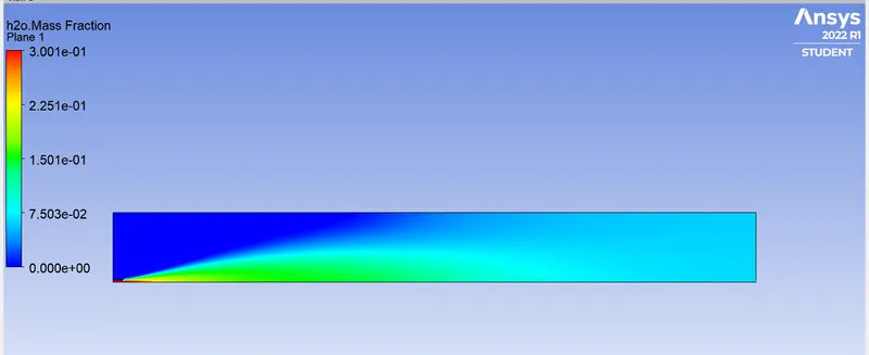
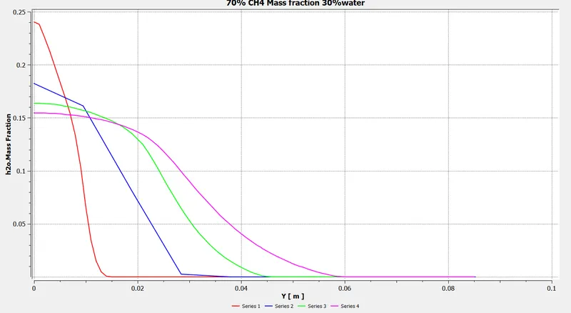
The H2O mass fraction is
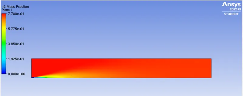
The N2 mass fraction is
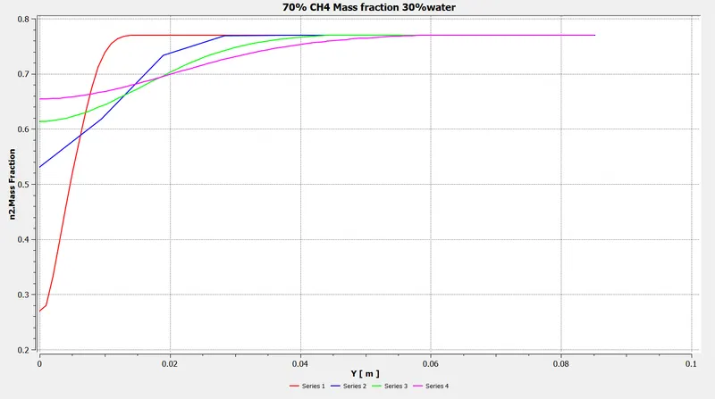
The O2 mass fraction is
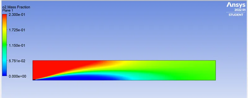
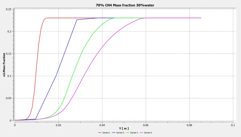
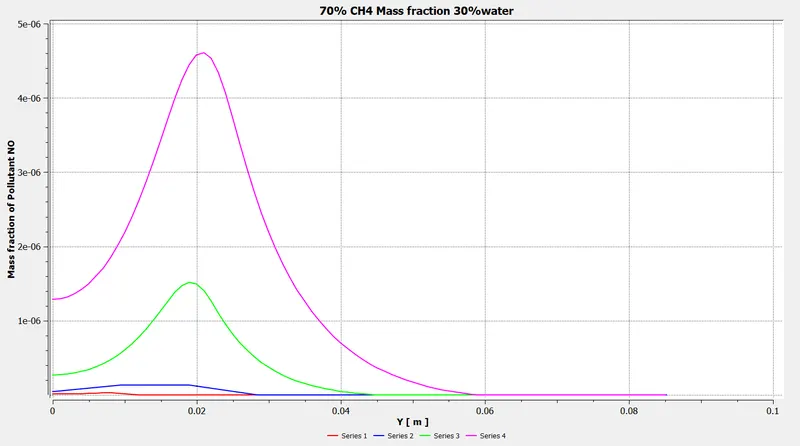
The pollutant NO mass fraction is
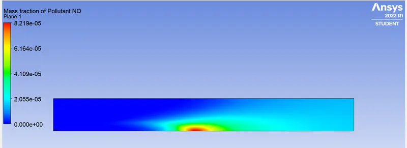
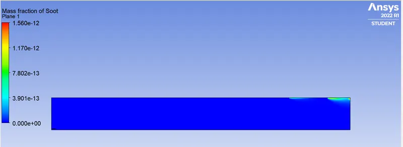
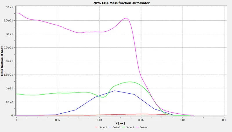
The soot mass fraction is
OBSERVATIONS:
We can see that from beginning, CH4 is burning from high a 1 to near at 0. But in real there are some unburnt carbon particles always remaining. Due to this incomplete combustion of hydrocarbons, generation of soot or fly ash is happening.
We see that the NOx emissions which are due to combustion of nitrogen present in air is 79%. Due to which we see N2 is maximum all over the contours.
We see a minor decrease in temperature from 0% water to 30% water usage.
We see a minor decrease in NOx emmisions from 0% water to 30% water usage.
We see a gradual decrease in soot from 0% water to 30% water usage.
Also as there is no ignition source for combustion. So the rate of reactions are controlled by turbulence mixing by eddy dissipation model. So with large eddy mixing time scale combustion starts when turbulence comes into picture.
CLAIMS:
As per the above observations we observe that the addition of water decreases NOx and soot formation.
Added water dilutes calories of generated energy, which reduces the temperature significantly, NOx cannot form in high concentrations.
We see small decrease in temperature. Reducing combustion temperature means avoiding stoichiometric ratio. If this is low, it generates lower concentration of thermal NOx.
So, these are the various technologies which must be modified so as to reduce the NOx and soot formation, which helps to meet the Regulations of Government and can reduce the harmful effects on environment and humans and wildlife.
CONCLUSION:
The simulation provides a complete temperature distribution along the model and contours for various species has been studied for different mass fractions.
By adding water, the pollutant soot and NOx pollutant are forming at the outlet and there is decrease with increase in water fraction.The plots for the same has been studied into.