Week 10 - Simulating Combustion of Natural Gas.
Objective:-
Part I
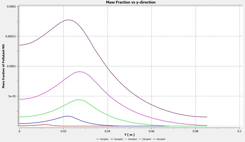
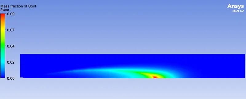
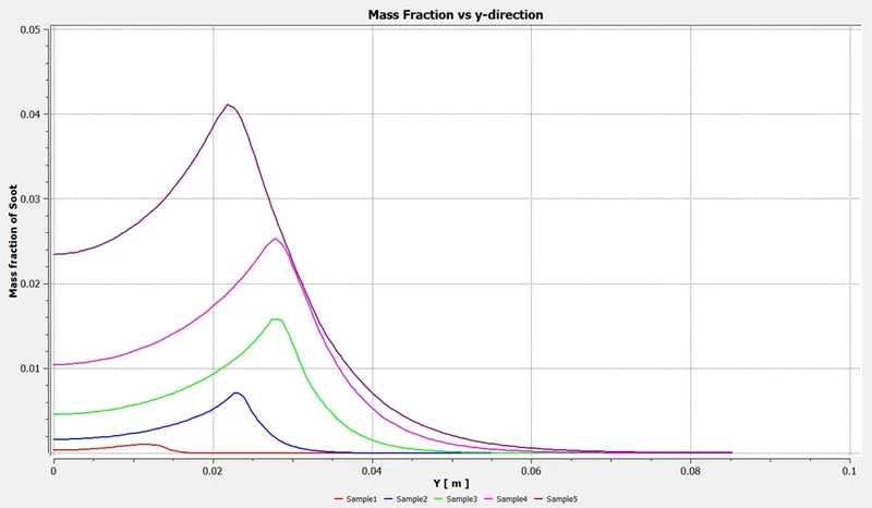
Perform a combustion simulation on the combustor model and plot the variation of the mass fraction of the different species’ in the simulation using line probes at different locations of the combustor. You need to plot for CO2, H2O, CH4, N2, O2, NOx emissions & Soot formation.
Part II
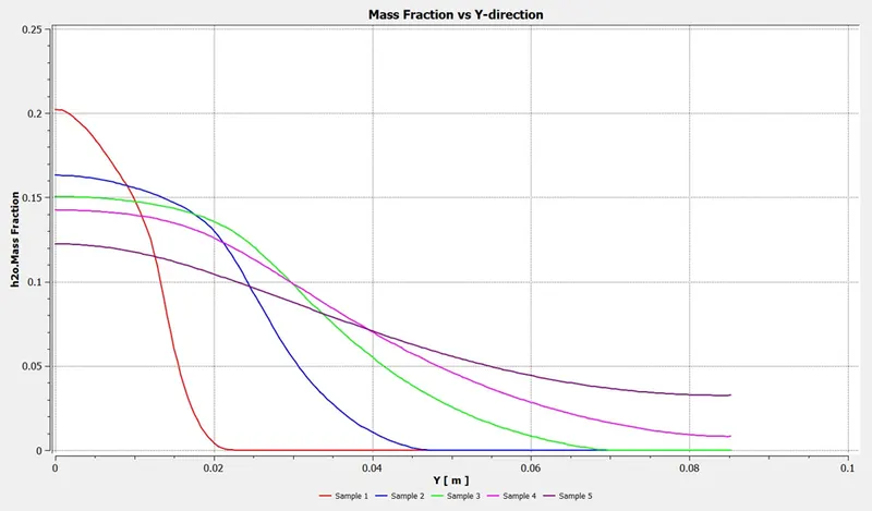
In this part, you need to add the water content in the fuel from 5% to 30% by mole and observe the effect of it on the results. It is necessary to provide line plots and contours to prove your claim.
Introduction:-
Combustion models for CFD refers to combustion models for computational fluid dynamics. Combustion is defined as a chemical reaction in which a hydrocarbon fuel reacts with an oxidant to form products, accompanied with the release of energy in the form of heat. Being the integral part of various engineering applications like: internal combustion engines, aircraft engines, rocket engines, furnaces and power station combustors, combustion manifests itself as a wide domain during the design, analysis and performance characteristics stages of the above-mentioned applications. With the added complexity of chemical kinetics and achieving reacting flow mixture environment, proper modelling physics has to be incorporated during computational fluid dynamic (CFD) simulations of combustion. Hence the following discussion presents a general outline of the various adequate models incorporated with the Computational fluid dynamic code to model the process of combustion.
Eddy dissipation model (EDM)
The eddy dissipation model is based on the concept that chemical reaction is fast relative to the transport processes in the flow. When reactants mix at the molecular level, they instantaneously form products. The model assumes that the reaction rate may be related directly to the time required to mix reactants at the molecular level.
By default, for the eddy dissipation model, it is sufficient that fuel and oxidant be available in the control volume for combustion to occur.
Because of the assumption of complete combustion, the eddy dissipation model may overpredict temperature under certain conditions (e.g., for hydrocarbon fuels in regions with fuel-rich mixture).
The eddy dissipation model was developed for use in a wide range of turbulent reacting flows covering premixed and diffusion flames. Because of its simplicity and robust performance in predicting turbulent reacting flows, this model has been widely applied in the prediction of industrial flames.
The finite-rate chemistry (FRC) model
The finite-rate chemistry model allows the computation of reaction rates described by the molecular interaction between the components in the fluid. It can be combined with the eddy dissipation model for flames where chemical reaction rates might be slow compared with the reactant mixing rates. The finite-rate chemistry model is best applied to situations where the chemical time scale is rate-limiting. This model can be used in conjunction with both laminar and turbulent flow.
The flamelet model
The flamelet model can provide information on minor species and radicals, such as CO and OH, and accounts for turbulent fluctuations in temperature and local extinction at high scalar dissipation rates, for the cost of solving only two transport equations. The model is only applicable for two-feed systems (fuel and oxidizer) and requires a chemistry library as input. The model can be used only for non-premixed systems.
The flamelet concept for non-premixed combustion describes the interaction of chemistry with turbulence in the limit of fast reactions (large Damköhler number). The combustion is assumed to occur in thin sheets with inner structure called flamelets. The turbulent flame itself is treated as an ensemble of laminar flamelets which are embedded into the flow field.
The main advantage of the flamelet model is that even though detailed information of molecular transport processes and elementary kinetic reactions are included, the numerical resolution of small length and time scales is not necessary. This avoids the well-known problems of solving highly nonlinear kinetics in fluctuating flow fields and makes the method very robust. Only two scalar equations have to be solved independent of the number of chemical species involved in the simulation. Information of laminar model flames are pre-calculated and stored in a library to reduce computational time (PDF table). On the other hand, the model is still restricted by assumptions like fast chemistry or the neglecting of different Lewis numbers of the chemical species.
The coupling of laminar chemistry with the fluctuating turbulent flow field is done by a statistical method. The PDF used can in principle be calculated at every point in the flow field by solving a PDF transport equation.
The most often mentioned advantage of this method is that the nonlinear chemical source term needs no modeling. Even though the method avoids some modeling which is necessary if using moment closure, it still requires modeling of some of the most important terms, in particular, the fluctuating pressure gradient term and the molecular diffusion term. If combustion occurs in thin layers as assumed here, the molecular diffusion term is closely coupled to the reaction term, and the problem of modeling the chemical source term is then shifted towards modeling the diffusion term.
Burning velocity model (BVM) and extended coherent flame model (ECFM)
The burning velocity model (BVM) and the extended coherent flame model (ECFM) model the propagation of a premixed or partially premixed flame by solving a scalar transport equation for the reaction progress. The BVM uses an algebraic correlation for modeling the turbulent burning velocity (propagation speed of the flame in turbulent flow). When using the ECFM, the turbulent burning velocity is closed by solving an additional transport equation for the flame surface density.
Procedure:-
Geometry
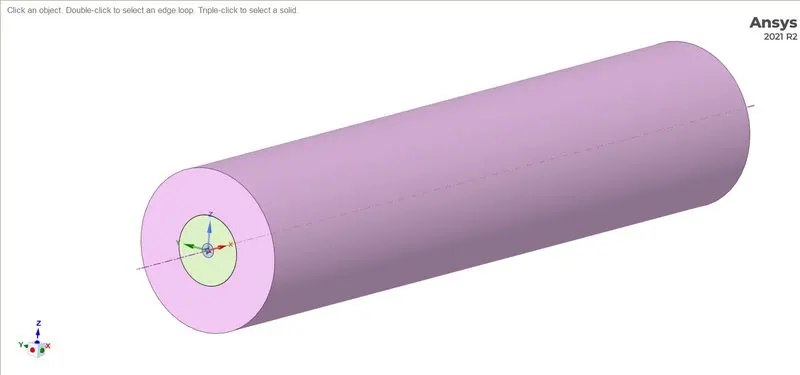
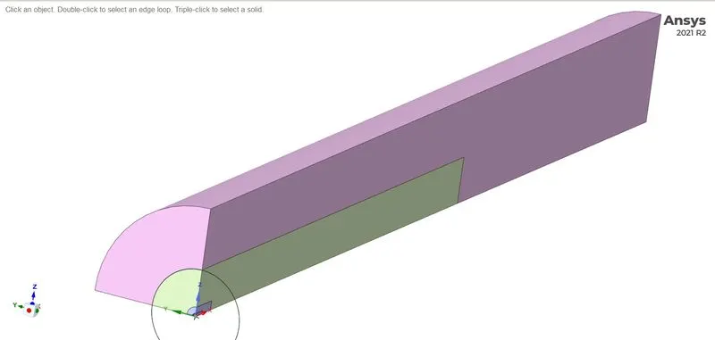
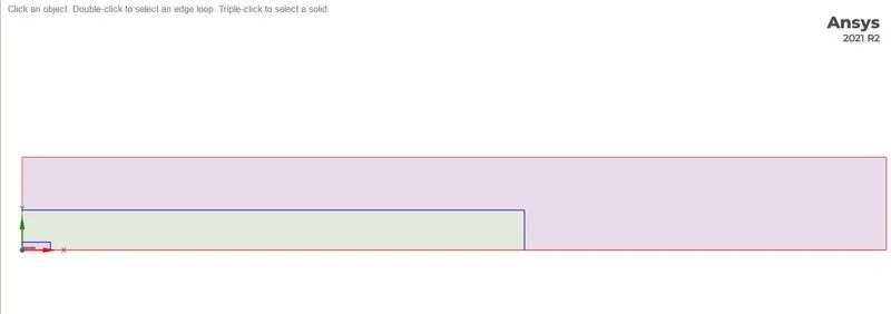
A 2-D analysis will be performed, since the body is axisymmetric. Extracting the area from the 3-D model by splitting the model. Taking only the 1/4th part of the model.
Meshing
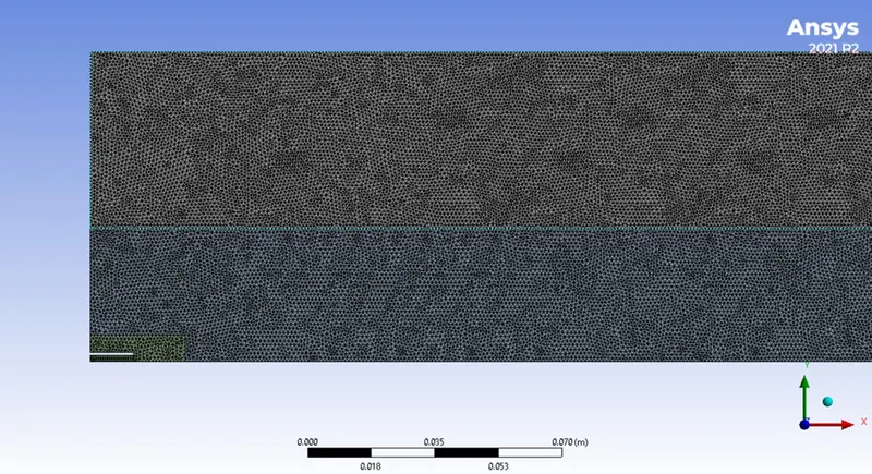
Meshing is done with an element size of 1mm and capture proximity is also used with number of cells as 3
Named sections
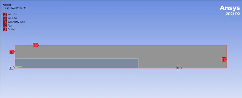
Setup
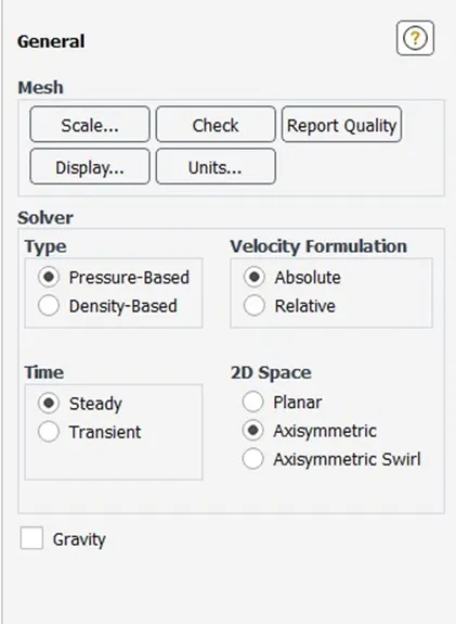
- Solver- Pressure Based
- Steady state, Absolute and Axisymmetric
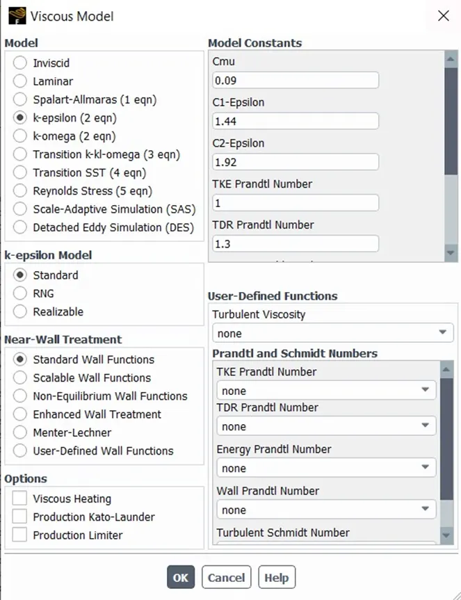
- Viscous Turbulence model- Standard K-epsilon model with Standard Wall Functions
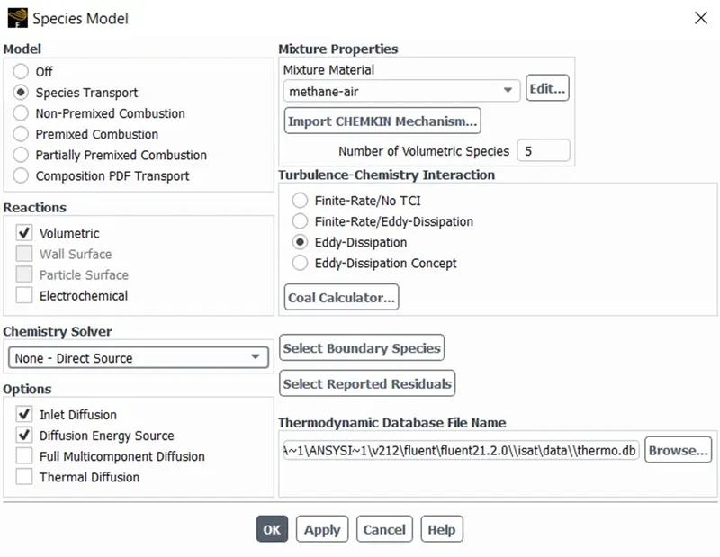
- Species model turned on. Volumetric option is activated
- For Fuel, Methane-Air -2step fuel model is selected
- For turbulence- Chemistry interaction, eddy-dissipation function is selected
- For capturing NOx and soot formation, NOx and soot model is activated
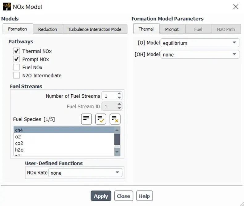
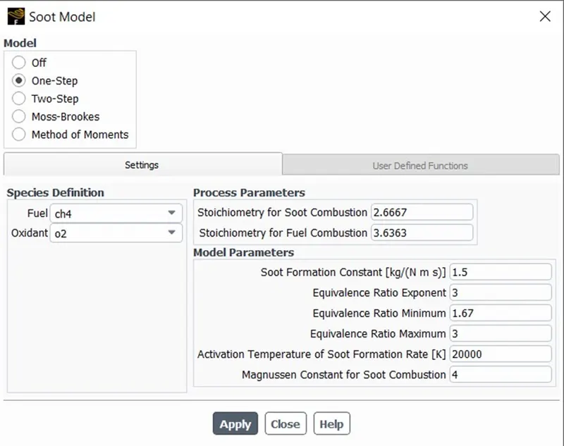
Boundary Conditions
- Case 1
Velocity of air at inlet is kept at 0.5 m/s with a temperature of 300k with species of 0.23 mass fraction of `O_2`. For Fuel inlet, velocity is 80 m/s and temperature of 300k with 1 as mass fraction for species `CH_4`
- Case 2
There will be addition of water of about 5, 15, 25, 30% in fuel. The corresponding change will only be at the fuel inlet.
Mass Fraction of `H_2O` with `CH_4` is given below
|
% |
5 |
15 |
25 |
30 |
|
Mass fraction of `H_2O` |
0.05 |
0.15 |
0.25 |
0.3 |
|
Mass fraction of `CH_4` |
0.95 |
0.85 |
0.75 |
0.7 |
Hybrid initialization is done and run for 1000 iterations
Results:-
Case 1
Residuals
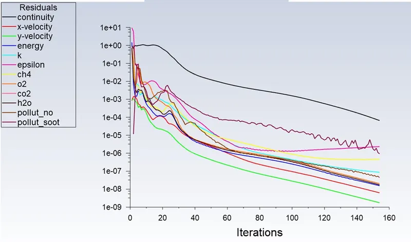
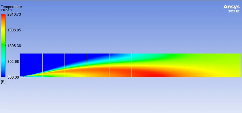
Temperature contour
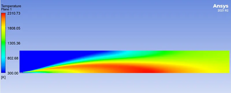
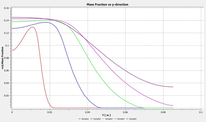
The sample is taken from the lines drawn on the temperature contour and is shown below
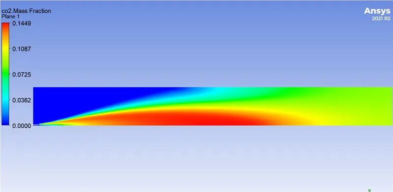
Mass Fraction of `CO_2`
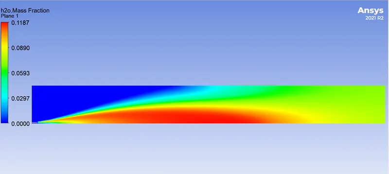
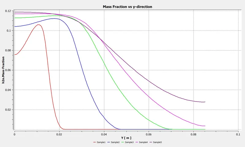
Mass Fraction of `H_2O`
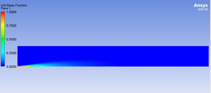
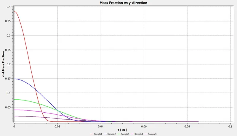
Mass Fraction of `CH_4`
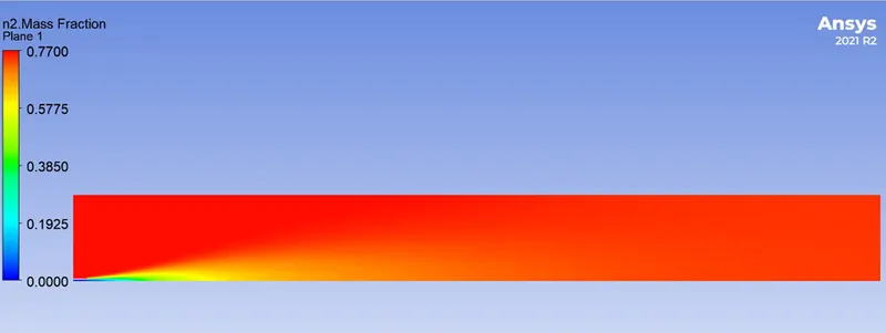
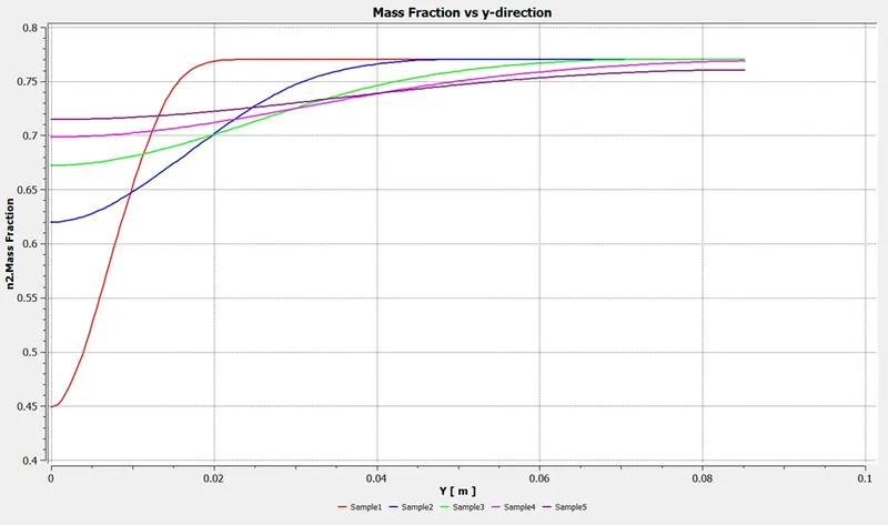
Mass Fraction of `N_2`
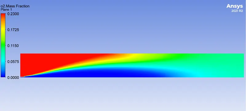
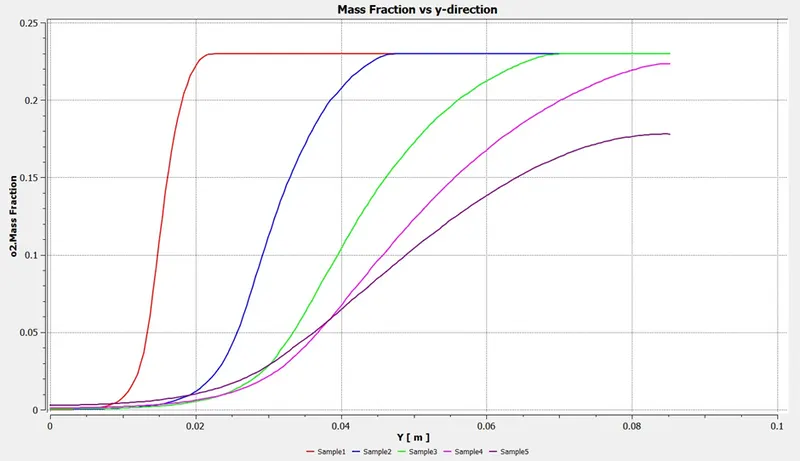
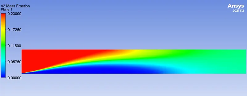
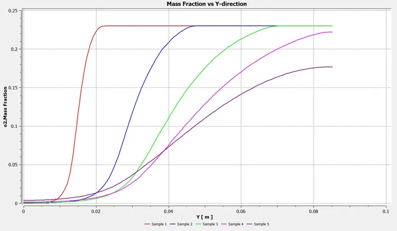
Mass Fraction of `O_2`
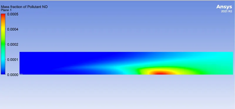
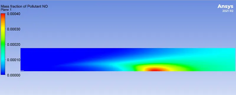
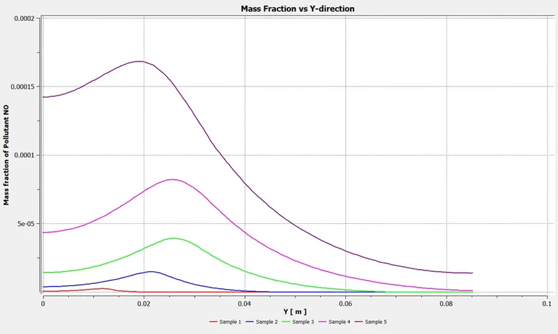
Mass Fraction of NOx
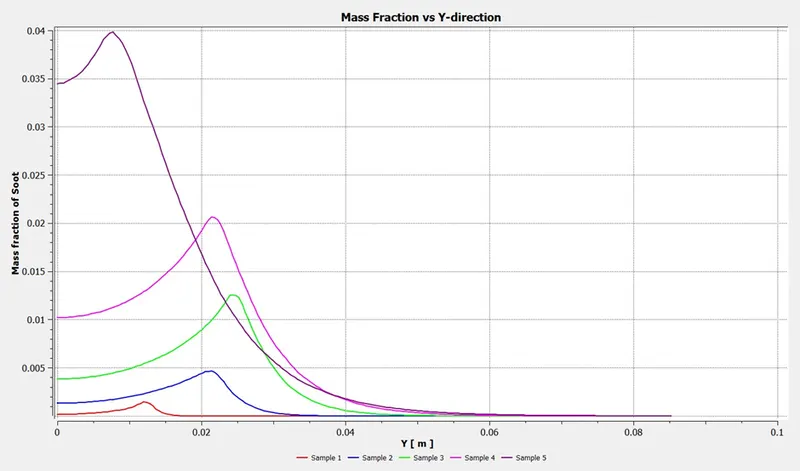
Mass Fraction of Soot
Case 2
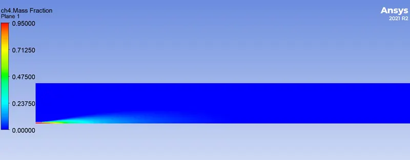
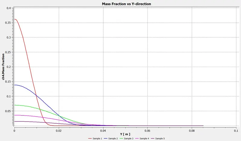
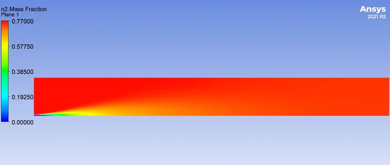
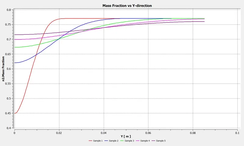
5% water content in the Fuel
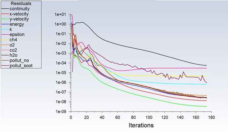
Residual
Mass Fraction of `CO_2`
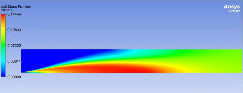
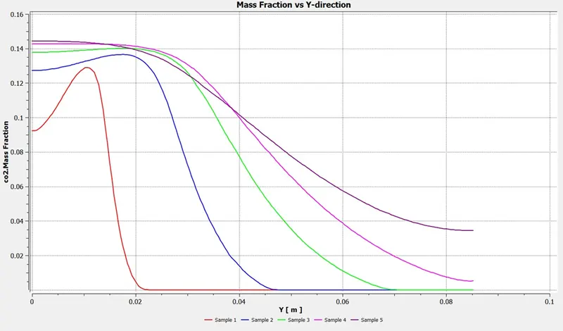
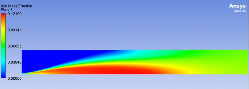
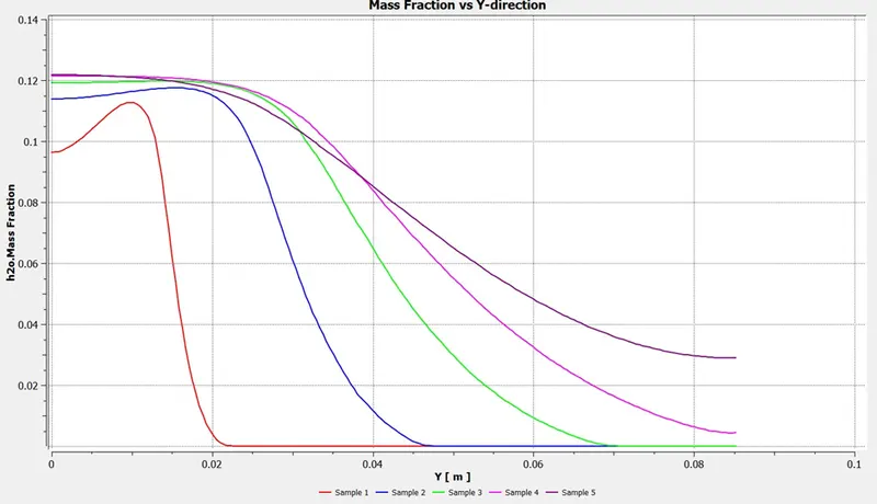
Mass Fraction of `H_2O`
Mass Fraction of `CH_4`
Mass Fraction of `N_2`
Mass Fraction of `O_2`
Mass Fraction of NOx
Mass Fraction of Soot
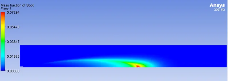
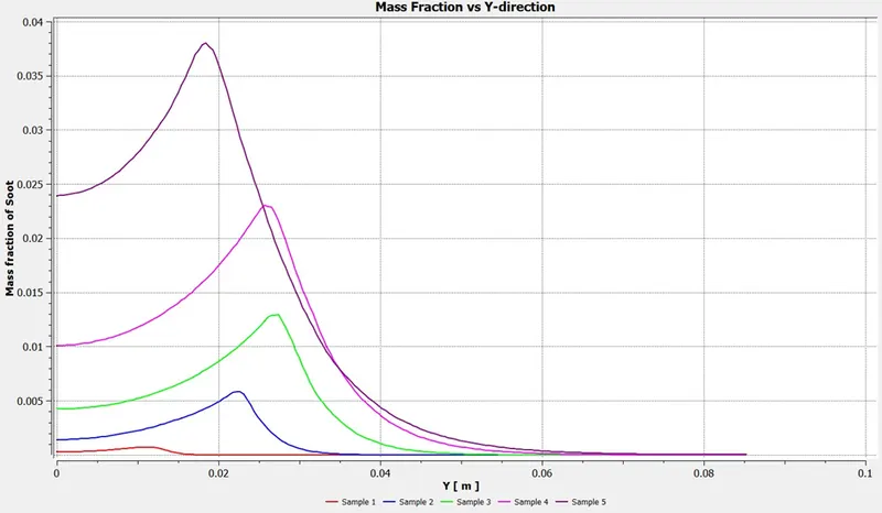
15% water content in the Fuel
Residual
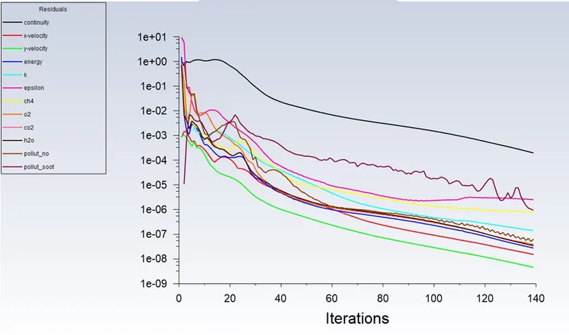
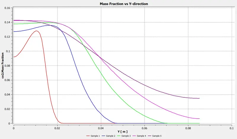
Mass Fraction of `CO_2`
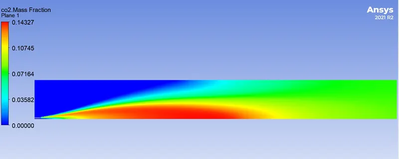
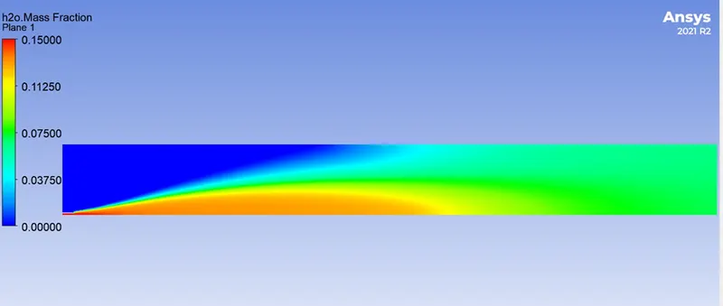
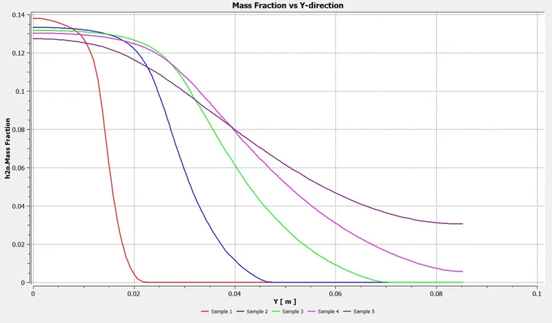
Mass Fraction of `H_2O`
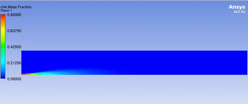
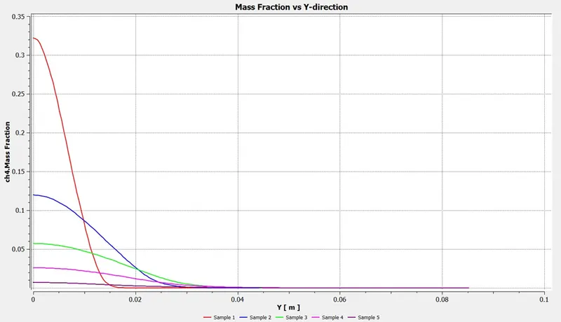
Mass Fraction of `CH_4`
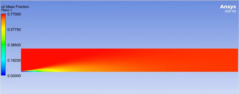
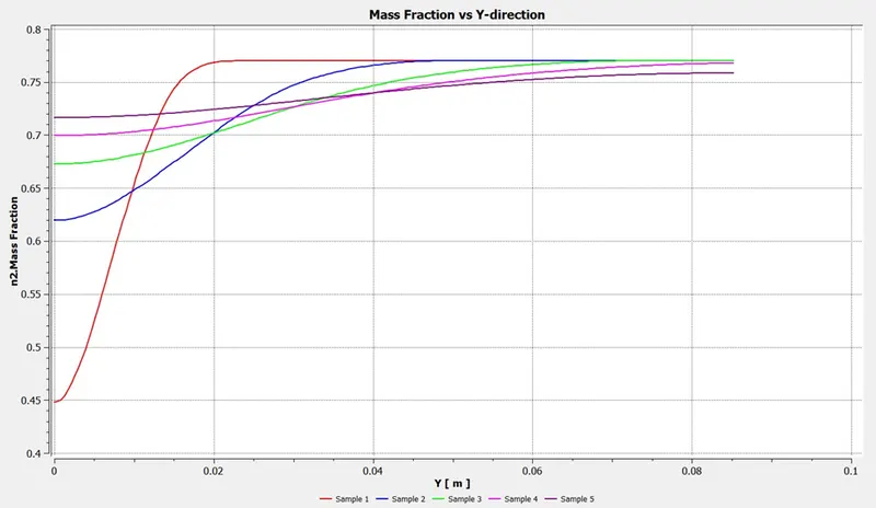
Mass Fraction of `N_2`
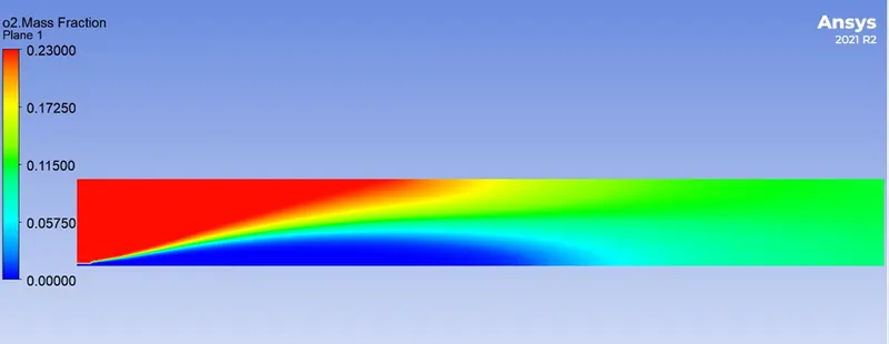
Mass Fraction of `O_2`
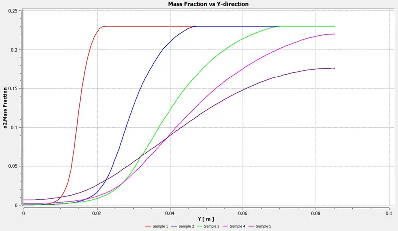
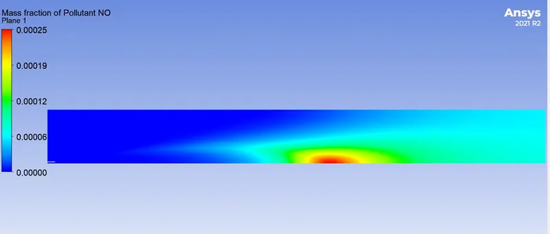
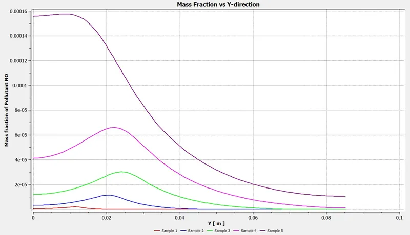
Mass Fraction of NOx
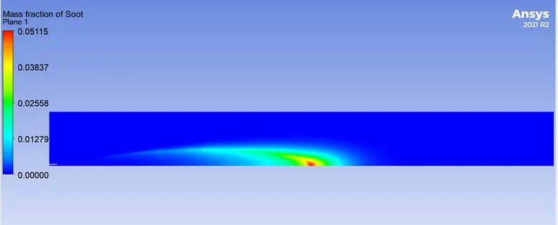
Mass Fraction of Soot
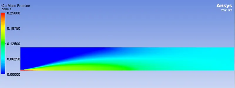
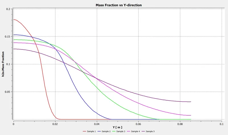
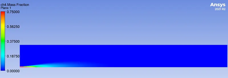
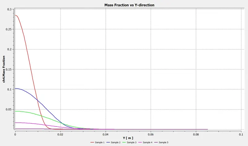
25% water content in the Fuel
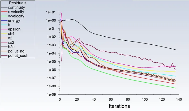
Residual
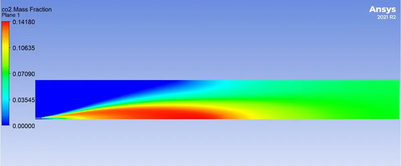
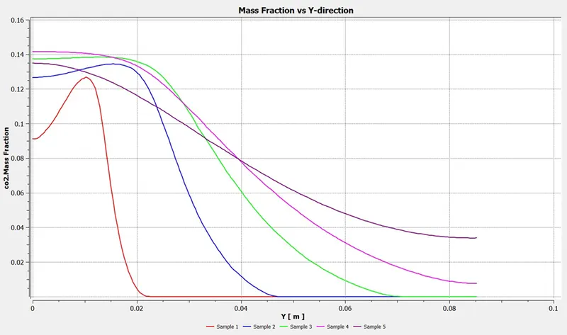
Mass Fraction of `CO_2`
Mass Fraction of `H_2O`
Mass Fraction of `CH_4`
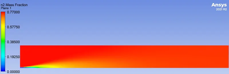
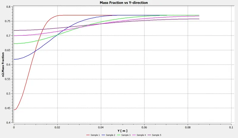
Mass Fraction of `N_2`
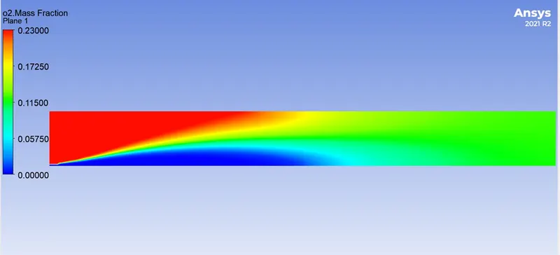
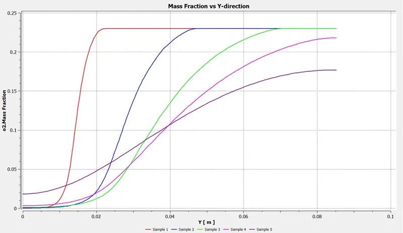
Mass Fraction of `O_2`
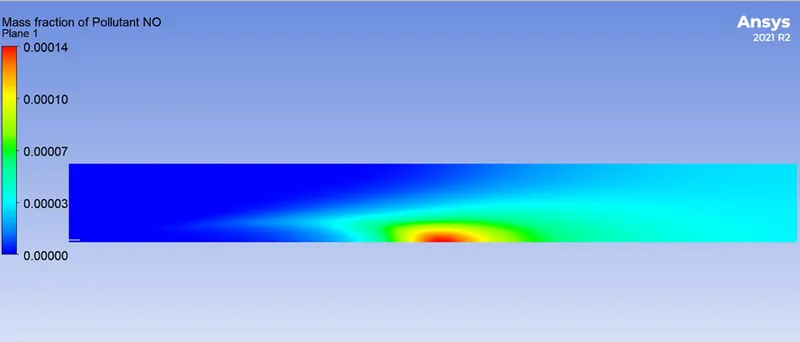
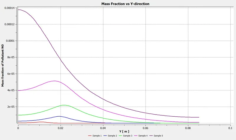
Mass Fraction of NOx
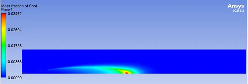
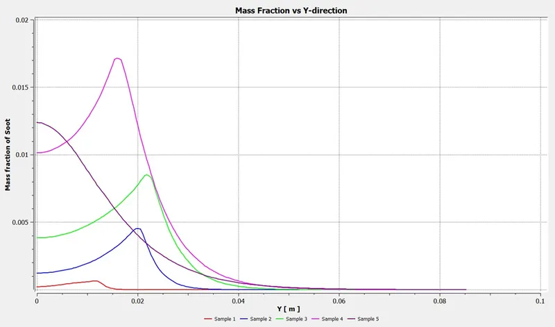
Mass Fraction of Soot
30% water content in the Fuel
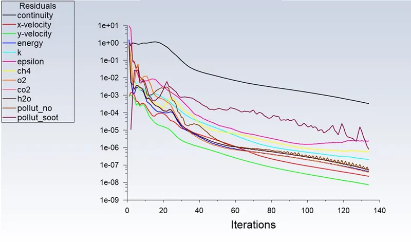
Residual
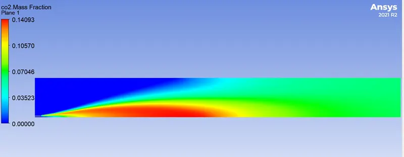
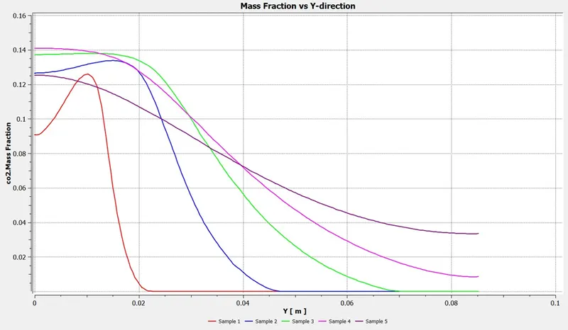
Mass Fraction of `CO_2`
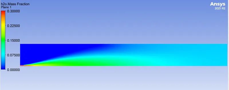
Mass Fraction of `H_2O`
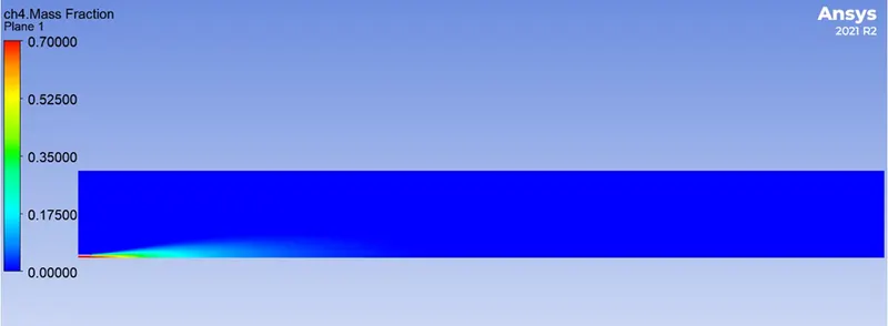
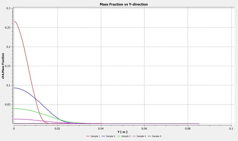
Mass Fraction of `CH_4`
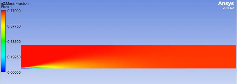
Mass Fraction of `N_2`
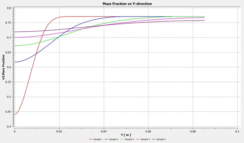
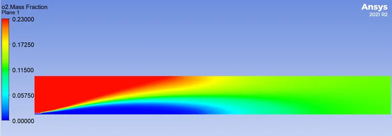
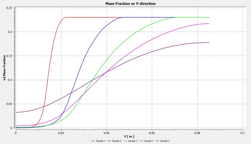
Mass Fraction of `O_2`
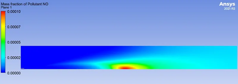
Mass Fraction of NOx
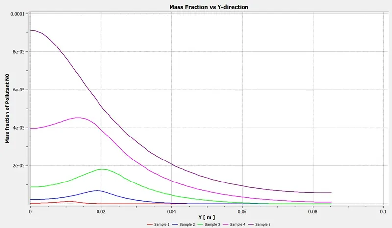
Mass Fraction of Soot
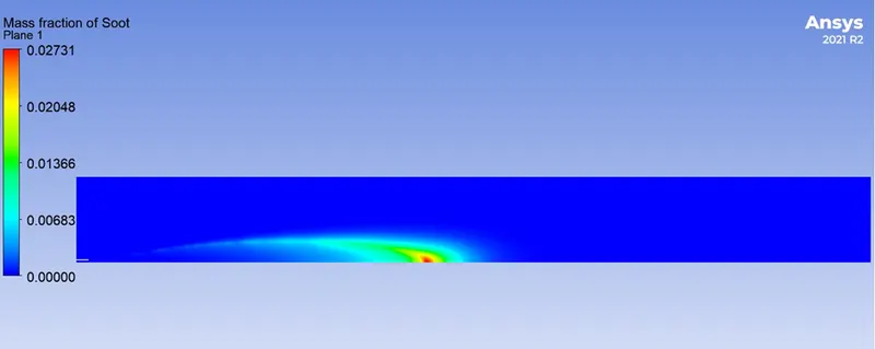
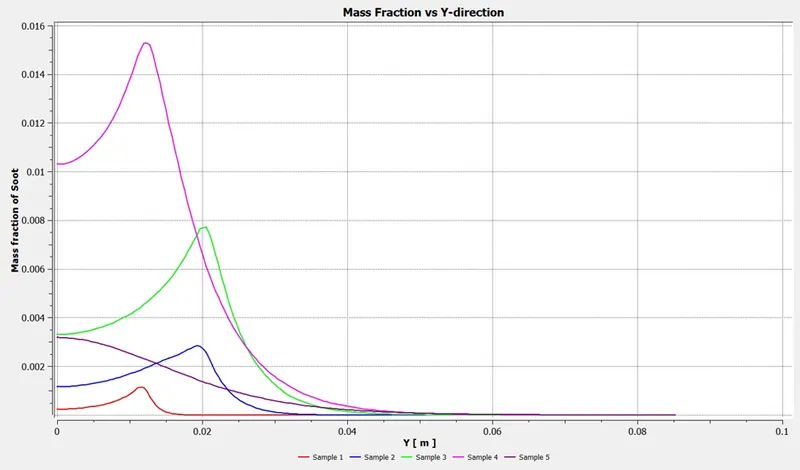
|
% water in fuel |
Mass fraction of NOx |
Mass fraction of soot |
|
5 |
`1.16*10^-4` |
`1.962*10^-5` |
|
15 |
`6.5181*10^-5` |
`2.8066*10^-6` |
|
25 |
`3.2736*10^-5` |
`3.3015*10^-7` |
|
30 |
`2.1941*10^-5` |
`9.7333*10^-8` |
Conclusion:-
From the above result it can be seen that as the water content in the fuel increases, the mass fraction of NOx pollutant and the mass fraction of soot decreases.
The results obtained from the simulation shows that the addition of water into the fuel not only decreases the temperature of the combustor but also helps in reducing the mass fraction of pollutants i.e NOx and soot