Full Hydrodynamic Simulation of a Port Fuel Injection Engine using CONVERGE CFD
I. Aim
To perform full hydrodynamic simulation of a port fuel injected engine and calculate the following parameters:
i. Compression ratio
ii. Combustion efficiency
iii. Engine power
iv. Engine torque
II. Given
i. PFI geometry
ii. Design inputs
III. Theory
Spray modeling: Modeling the fuel spray in the intake port is a very crucial step in the process of simulating port fuel injected (PFI) engine. In order to correctly model the spray, the following involved physical phenomena must be modeled accurately:
i. Liquid atomization
ii. Drop breakup
iii. Drop collision
iv. Drop coalescence
v. Turbulent dispersion
vi. Drop evaporation
CONVERGE models the spray using parcels, each of which represents a collection of identical drops (having the same geometric and flow properties). These parcels represent the entire spray field statistically. CONVERGE solves for the flow and geometric properties of these parcels (and not of the individual drops). For liquid sprays, CONVERGE uses Lagrangian solver to model the discrete parcels and Eulerian solver to model the continuous fluid domain. Heat, momentum and mass transfer between the discrete phase and the continuous phase are modeled using source terms in the transport equations. The parcels undergo all the physical processes that are involved in the development of sprays:
i. Primary breakup: The breakup of initially defined parcels into tiny parcels due to their interaction with the gas phase.
ii. Secondary breakup: The tiny parcels, generated due to primary breakup, can undergo another breakup depending upon their size and the hydrodynamic conditions.
iii. Drop drag: Due to their interaction with the surrounding gas phase, the parcels experience drop drag which affects their shapes.
iv. Collision and coalescence: The tiny parcels can collide with other parcels and can even merge with them.
v. Turbulent dispersion: The presence of fluctuating velocity components in the gas phase affect the dispersion of parcels.
vi. Evaporation: The tiny parcels undergo combustion and get evaporated.
Spray modeling setup in CONVERGE
i. Parcel distribution: CONVERGE assumes that the injection is conical for solid cone sprays, and provides two different types of parcel distribution:
(a) Cluster parcels near the cone center
(b) Distribute the parcels uniformly throughout the cone
ii. Evaporation model: CONVERGE provides the following two evaporation models to evaluate the rate of change of radius:
(a) Frossling model
(b) Chiang model
CONVERGE provides three different ways of simulating multi-component vaporization as follows:
(a) Source specified species: Parcels evaporate to the specified species.
(b) Source all composite parcel species: Multi-component liquid species evaporate into the composite species defined in composite.in.
(c) Source all base parcel species: Multi-component liquid species evaporate into the base parcel species.
For each parcel, CONVERGE assumes a uniform temperature distribution unless the parcel radius exceeds a cut-off radius (specified by the user). In that case, one dimensional heat equation along the radial coordinate is solved to obtain the temperature field.
iii. Spray penetration: Spray penetration is animportant parameter in both experimental and computational analysis of sprays. CONVERGE calculates and writes the liquid penetration length (LPL) and vapor penetration length (VPL) at each output interval.
LPL is the distance measured along the nozzle axis from the point of injection to the point where the mass fraction of the spray mass, with respect to the total liquid mass in the domain, reaches the value specified by the user (default 0.98).
VPL is the distance measured between the center of the nozzle and the cell center of the last cell (located along the nozzle-axis) which satisfies the following criteria:
(a) The vapor mass fraction in the cell exceeds a certain minimum value (specified by the user).
(b) The cell size is smaller than the user-specified bin size.
iv. Mass diffusivity constants
The mass diffusivity of liquid vapor in air is given by:
`D=(1.293D_0)/rho_(gas)(T_(gas)/273)^(n_0-1)`
The values of constants `n_0` and `D_0` are provided by the user. For popular fuels, CONVERGE provides these constants.
v. Collision/Coalescence: CONVERGE provides three collision models:
(a) No collision
(b) O'Rourke numerical algorithm
(c) NTC numerical algorithm
In addition to this the following two collision outcomes may also be specified by the user:
(a) O'Rourke collision outcomes
(b) Post collision outcomes
CONVERGE also provides an option to use collision mesh for performing collision calculations. A collision mesh is an adaptive mesh which is independent of the gas phase grid and is used only for collision calculations. It allows the parcels to collide across grid cells. This is helpful in eliminating the grid sensitivity of results.
vi. Drop drag: CONVERGE provides the following three options for including the effect of drag on the liquid parcels as they move through the gas phase:
(a) No drop drag: The influence of drag is completely ignored.
(b) Spherical drop drag: The drag coefficient calculation assumes the parcels to be perfect spheres.
(c) Dynamic drag model: The drag coefficient calculation accounts for variations in parcel shape. The parcel distortion is determined by TAB model.
vii. Drop/Wall interaction: CONVERGE includes the following three models to capture the parcel-wall interaction:
(a) Rebound/slide: Parcels rebound or slide along the wall after impingement.
(b) Wall film: Parcel actions are calculated using a hybrid approach based on particle-based quantities or film-based quantities. If this model is employed then a film splash model must also be used out of the following two options:
b.1. O'Rourke: The possible parcel outcomes are based on the Weber number, film thickness and viscosity or simply the Weber number.
b.2. Kuhnke: The possible parcel outcomes are rebound, splash, thermal breakup and deposition.
(c) Vanish: The parcels vanish after hitting a wall boundary.
viii. Injectors: CONVERGE allows the user to define the following:
(a) Injected species: Parcel species and its mass fraction are defined for the injectors.
(b) Injection rate-shape: Rate-shape of the injection process is defined using normalized mass of the injected species and normalized time.
(c) Instability models: The instabiity models dictate the process of spray breakup. They determine various important parameters such as: droplet size after the breakup process, time scale of the breakup process etc. CONVERGE provides the following models:
c.1. Kelvin-Helmholtz (KH) model
c.2. Rayleigh-Taylor (RT) model
c.3. Linearized Instability Sheet Atomization (LISA) model
c.4. Taylor Analogy Breakup (TAB) model
c.5. Discharge coefficient model
(d) Injection process: CONVERGE allows the user to specify the following details related to the injection process:
d.1. Injection temporal type: CYCLIC or SEQUENTIAL
d.2. Start of injection in crank angle
d.3. Injection duration in crank angle
d.4. Total injected mass
d.5. Total number of injected parcels per nozzle
d.6. Injection drop distribution
d.7. Temperature
d.8. Turbulent kinetic energy
d.9. Turbulent dissipation
(e) Nozzles: CONVERGE allows the user to specify the type of injection spray (Hollow cone spray or Solid cone spray). Depending on the problem, the number of nozzles can be added and configured separately. For each nozzle, the user can specify details such as: nozzle diameter, circular injection radius, spray cone angle, location and orientation etc.
Combustion modeling: Combustion is a chemical process during which heat energy is released by the virtue of chemical reaction between a fuel and an oxidizer. Combustion modeling is one of the most important steps involved in simulating engineering devices that utilize thermal energy released during combustion process. CONVERGE provides both detailed chemistry solver (SAGE) and simplified combustion models to capture the combustion process.
SAGE chemistry solver
It uses the local conditions to calculate reaction rates based on the principles of chemical kinetics. It computes the rate of change of mass fraction of different species, involved in the combustion chemical reactions, using the rate law. All the necessary details related to the different chemical reactions involved in the combustion process are available in a reaction mechanism file. The chemistry solver imports this mechanism file and solves a system of ordinary differential equations using CVODES (general ODE solver) to obtain the rate of change of mass fraction of each species (present in the mechanism file). These terms are added as source terms in the transport equations of the respective species. In this way the transport solver and the chemistry solver are coupled via source terms. The general form of species transport equation including the source term is given below:
`(delbar(rho)tilde(Y)_m)/(delt)+(delbar(rho)tilde(u)_jtilde(Y)_m)/(delx_j)=del/(delx_j)(bar(rho)D_t(deltilde(Y)_m)/(delx_j))+tilde(dot(omega))_m`
where `tilde(dot(omega))_m` is the source term.
The mechanism file contains elementary reactions in the Arrhenius format wherein the rate of forward reactionis given by the Arrhenius equation as given below:
`k_f=A_rT^be^(-E_r/(RT))` where:
`A_r`: Pre-exponential factor
`E_r`: Activation energy
`b`: Temperature exponent
`R`: Universal gas constant
The reverse reaction rate can be specified by the user or can be calculated from the equilibrium coefficient, which is determined using the properties available in therm.dat.
SAGE acceleration options
As described above SAGE solves for detailed chemistry in every computational cell which can be quite computationally expensive. To overcome this issue CONVERGE provides the following acceleration options:
i. Using Start time and End time to limit SAGE to specific time intervals.
ii. Limit SAGE to specific regions.
iii. Increase the Minimum cell temperature and Minimum HC species mole fraction parameters to reduce the number of cells in which the combustion calculations are performed.
iv. The Re-solve option should be set to: Only re-solve if temperature changes by specified value.
v. Select "Use analytical Jacobian" to pass an analytically calculated Jacobian to the solver.
vi. Enable the multizone or adaptive zone option to reduce the number of SAGE calculations by:
(a) Grouping the computational cells together into bins (zones)
(b) Calculating average quantities
(c) Invoking the SAGE solver once per bin instead of once per cell
(d) Mapping the solved quantities to all cells in the bin
(e) Enable the option "Conserve `NO_x` during species remap" to allow remapping using nitrogen atoms and thus improve `NO_x` predictions
Apart from the SAGE solver, which solves for the detailed chemistry, CONVERGE provides the following simplified combustion models:
i. Non-premixed turbulent combustion models
i.i. Characteristic Time Combustion (CTC)
i.ii. Shell Ignition
i.iii. Chemical Equilibrium (CEQ)
i.iv. Representative Interactive Flamelet (RIF)
i.v. Extended Coherent Flame Model with the 3Z mixing model (ECFM3Z)
ii. Premixed turbulent combustion models
ii.i. Chemical Equilibrium (CEQ)
ii.ii. G-Equation
ii.iii. Extended Coherent Flame Model (ECFM)
ii.iv. Flamelet Generated Manifold (FGM)
IV. Case setup
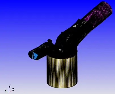
1. Geometry
The geometry used for simulation is shown in the figure attached below.
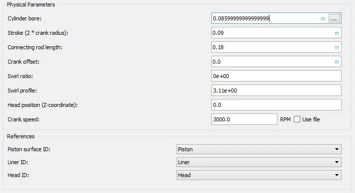
2. Application type
A crank angle based IC engine simulation is performed with the following settings:
3. Materials
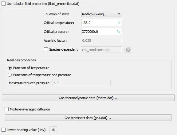
3.1. Gas simulation
The following settings are used for gas simulation:
3.2. Parcel simulation
Iso-octane parcels are used to mimic the gasoline fuel spray. This choice is made based on the thermophysical properties i.e. the species whose properties most closely resemble that of the fuel is selected.
3.3. Global transport parameters
Turbulent Prandtl number: 0.9
Turbulent Schmidt number: 0.78
3.4. Reaction mechanism
A reaction mechanism compatible with gasoline combustion, proposed by Ming Jia and Maozhao Xie, is used. The mechanism is based on the oxidation of iso-octane. Hence the fuel is iso-octane and the oxidizer is air (77% Nitrogen and 23% Oxygen by mass fractions). Additionally since the oxidation is assumed to be stoichiometric, the final products (after combustion) include nitrogen gas, water vapor and carbon dioxide.
The thermophysical properties of different species involved in the reaction mechanism are available in the therm.dat file.
3.5. Species
The parcel species are defined as iso-octane.
4. Simulation Parameters
4.1. Run parameters
Solver: Transient
Temporal type: Crank angle-based engine simulation
Gas flow solver: Compressible
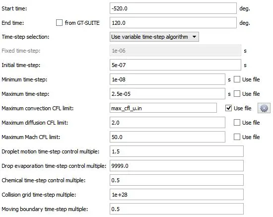
4.2. Simulation time parameters
4.3. Solver parameters
Navier-Stokes solver scheme: PISO
Navier-Stokes solver type: Density-based
5. Boundary conditions
The following boundary conditions are imposed on the different boundaries:
i. Piston:
Velocity boundary condition:
Boundary type: WALL
Wall motion type: Translating
Surface movement: MOVING
Law of the wall; Piston motion
Temperature boundary condition:
Law of the wall; 450K
Heat model:
O'Rourke and Amsden
Turbulent Kinetic Energy boundary condition:
Zero normal gradient
Turbulent Dissipation boundary condition:
Wall model
Region Name: Cylinder
ii. Liner:
Velocity boundary condition:
Boundary type: WALL
Wall motion type: Stationary
Surface movement: FIXED
Law of the wall
Temperature boundary condition:
Law of the wall; 450K
Heat model:
O'Rourke and Amsden
Turbulent Kinetic Energy boundary condition:
Zero normal gradient
Turbulent Dissipation boundary condition:
Wall model
Region Name: Cylinder
iii. Head:
Velocity boundary condition:
Boundary type: WALL
Wall motion type: Stationary
Surface movement: FIXED
Law of the wall
Temperature boundary condition:
Law of the wall; 450K
Heat model:
O'Rourke and Amsden
Turbulent Kinetic Energy boundary condition:
Zero normal gradient
Turbulent Dissipation boundary condition:
Wall model
Region Name: Cylinder
iv. Spark plug:
Velocity boundary condition:
Boundary type: WALL
Wall motion type: Stationary
Surface movement: FIXED
Law of the wall
Temperature boundary condition:
Law of the wall; 550K
Heat model:
O'Rourke and Amsden
Turbulent Kinetic Energy boundary condition:
Zero normal gradient
Turbulent Dissipation boundary condition:
Wall model
Region Name: Cylinder
v. Spark plug electrode
Velocity boundary condition:
Boundary type: WALL
Wall motion type: Stationary
Surface movement: FIXED
Law of the wall
Temperature boundary condition:
Law of the wall; 600K
Heat model:
O'Rourke and Amsden
Turbulent Kinetic Energy boundary condition:
Zero normal gradient
Turbulent Dissipation boundary condition:
Wall model
Region Name: Cylinder
vi. Exhaust ports
Velocity boundary condition:
Boundary type: WALL
Wall motion type: Stationary
Surface movement: FIXED
Law of the wall
Temperature boundary condition:
Law of the wall; 500K
Heat model:
O'Rourke and Amsden
Turbulent Kinetic Energy boundary condition:
Zero normal gradient
Turbulent Dissipation boundary condition:
Wall model
Region Name: Exhaust system
vii. Exhaust outflow:
Pressure boundary condition: 101325Pa
Velocity boundary condition: Zero normal gradient
Temperature backflow: 800K
Species backflow: Calculated based on the stoichiometric coefficients of the product species in the reaction given below:
`C_8H_18+12.5(O_2+3.76N_2)=8CO_2+9H_2O+(12.5times3.76)N_2`
Number of moles of `CO_2`=8mol
Gram molecular weight of `CO_2`=44.01g/mol
Mass of `CO_2`=352.08g
Number of moles of `H_2O`=9mol
Gram molecular weight of `H_2O`=18.01528g/mol
Mass of `H_2O`=162.1375g
Number of moles of `N_2`=47mol
Gram molecularweight of `N_2`=28.0134g/mol
Mass of `N_2`=1316.63g
Total mass of the products= Mass of `CO_2`+ Mass of `H_2O` + Mass of `N_2`=352.08g+162.1375g+1316.63g=1830.847g
Mass fraction of `CO_2`=0.192304
Mass fraction of `H_2O`=0.088559
Mass fraction of `N_2`=0.719137
Turbulent Kinetic Energy backflow: Intensity (fraction)=0.02
Turbulent Dissipation backflow: Length scale (m)=0.003m
Region Name: Exhaust system
viii. Exhaust valve top:
Velocity boundary condition:
Boundary type: WALL
Wall motion type: Translating
Surface movement: MOVING
Law of the wall
For the exhaust valve motion, user defined file is used.
Temperature boundary condition:
Law of the wall; 525K
Heat model:
O'Rourke and Amsden
Turbulent Kinetic Energy boundary condition:
Zero normal gradient
Turbulent Dissipation boundary condition:
Wall model
Region Name: Exhaust system
ix. Exhaust valve angle:
Velocity boundary condition:
Boundary type: WALL
Wall motion type: Translating
Surface movement: MOVING
Law of the wall
For the exhaust valve motion, user defined file is used.
Temperature boundary condition:
Law of the wall; 525K
Heat model:
O'Rourke and Amsden
Turbulent Kinetic Energy boundary condition:
Zero normal gradient
Turbulent Dissipation boundary condition:
Wall model
Region Name: Exhaust system
x. Exhaust valve bottom:
Velocity boundary condition:
Boundary type: WALL
Wall motion type: Translating
Surface movement: MOVING
Law of the wall
For the exhaust valve motion, user defined file is used.
Temperature boundary condition:
Law of the wall; 525K
Heat model:
O'Rourke and Amsden
Turbulent Kinetic Energy boundary condition:
Zero normal gradient
Turbulent Dissipation boundary condition:
Wall model
Region Name: Cylinder
xi. Intake port:
Velocity boundary condition:
Boundary type: WALL
Wall motion type: Stationary
Surface movement: FIXED
Law of the wall
Temperature boundary condition:
Law of the wall; 425K
Heat model:
O'Rourke and Amsden
Turbulent Kinetic Energy boundary condition:
Zero normal gradient
Turbulent Dissipation boundary condition:
Wall model
Region Name: Intake system
xii. Intake port B:
Velocity boundary condition:
Boundary type: WALL
Wall motion type: Stationary
Surface movement: FIXED
Law of the wall
Temperature boundary condition:
Law of the wall; 425K
Heat model:
O'Rourke and Amsden
Turbulent Kinetic Energy boundary condition:
Zero normal gradient
Turbulent Dissipation boundary condition:
Wall model
Region Name: Intake system2
xiii. Intake (Inflow boundary):
Pressure boundary condition: 101325Pa
Velocity boundary condition: Zero normal gradient
Temperature boundary condition: 363K
Species boundary condition: Air
Mass fraction of `N_2`=0.77
Mass fraction of `O_2`=0.23
Turbulent Kinetic Energy boundary condition: Intensity (fraction)=0.02
Turbulent Dissipation boundary condition: Length scale (m)=0.003m
Region Name: Intake system
xiv. Intake valve top:
Velocity boundary condition:
Boundary type: WALL
Wall motion type: Translating
Surface movement: MOVING
Law of the wall
For the intake valve motion, user defined file is used.
Temperature boundary condition:
Law of the wall; 480K
Heat model:
O'Rourke and Amsden
Turbulent Kinetic Energy boundary condition:
Zero normal gradient
Turbulent Dissipation boundary condition:
Wall model
Region Name: Intake system2
xv. Intake valve angle:
Velocity boundary condition:
Boundary type: WALL
Wall motion type: Translating
Surface movement: MOVING
Law of the wall
For the exhaust valve motion, user defined file is used.
Temperature boundary condition:
Law of the wall; 480K
Heat model:
O'Rourke and Amsden
Turbulent Kinetic Energy boundary condition:
Zero normal gradient
Turbulent Dissipation boundary condition:
Wall model
Region Name: Intake system2
xvi. Intake valve bottom:
Velocity boundary condition:
Boundary type: WALL
Wall motion type: Translating
Surface movement: MOVING
Law of the wall
For the exhaust valve motion, user defined file is used.
Temperature boundary condition:
Law of the wall; 480K
Heat model:
O'Rourke and Amsden
Turbulent Kinetic Energy boundary condition:
Zero normal gradient
Turbulent Dissipation boundary condition:
Wall model
Region Name: Cylinder
6. Initial Conditions and Events:
The different volumetric regions created in the domain are:
i. Cylinder
Velocity: 0
Temperature: 1360K
Pressure: 185731Pa
Turbulent Kinetic Energy: 10`m^2//s^2`
Turbulent Dissipation: 20000`m^2//s^3`
Mass fraction of `CO_2`=0.192304
Mass fraction of `H_2O`=0.088559
Mass of `N_2`=0.719137
ii. Intake system
Velocity: 0
Temperature: 370K
Pressure: 101325Pa
Turbulent Kinetic Energy: 10`m^2//s^2`
Turbulent Dissipation: 20000`m^2//s^3`
Mass fraction of `O_2`=0.23
Mass fraction of `N_2`=0.77
iii. Exhaust system
Velocity: 0
Temperature: 1215K
Pressure: 103737Pa
Turbulent Kinetic Energy: 10`m^2//s^2`
Turbulent Dissipation: 20000`m^2//s^3`
Mass fraction of `CO_2`=0.192304
Mass fraction of `H_2O`=0.088559
Mass of `N_2`=0.719137
iv. Intake system2
Velocity: 0
Temperature: 390K
Pressure: 101325Pa
Turbulent Kinetic Energy: 10`m^2//s^2`
Turbulent Dissipation: 20000`m^2//s^3`
Mass fraction of `C_8H_18`=0.025508
Mass fraction of `O_2`=0.20157
Mass fraction of `N_2`=0.77292
In order to mimic the opening and closing of valves, CONVERGE creates disconnect triangles between the following pairs of regions:
i. Cylinder and Intake system2
ii. Cylinder and Exhaust system
The presence or absence of these disconnect triangles is controlled by events. Events are used to establish the nature of contact between two adjacent regions. The following events are defined:
i. Event 1:
Type: Cyclic (`720^o`)
Region A: Cylinder
Region B: Intake system2
Event: VALVE (Intake valve profile is used)
ii. Event 2:
Type: Cyclic (`720^o`)
Region A: Cylinder
Region B:Exhaust system
Event: VALVE (Exhaust valve profile is used)
iii. Event 3:
Type: Permanent
Region A: Intake system
Region B: Intake system2
Event: OPEN
7. Physical Models
7.1. Spray modeling
7.1.1. Parcel distribution: Parcels are distributed evenly throughout the solid cone.
7.1.2. Turbulent dispersion: For gasoline sprays O'Rourke model works quite well and hence is selected.
7.1.3. Evaporation model: Frossling model
7.1.4. Evaporation source: Source all base parcel species
7.1.5. Maximum radius for ODE droplet heating: 1000m (A very large number is selected on purpose to avoid solving the ODE for droplet heating. This speeds up the solution procedure)
7.1.6. Collision model: NTC collision model
7.1.7. Collision outcomes: Post collision outcomes
7.1.8. Collision mesh (Level of collision): 2
7.1.9. Drop drag model: Dynamic drop drag
7.1.10. Spray-wall interaction model: Wall film
7.1.11. Film splash model: O'Rourke (Based on Weber number, film thickness and viscosity)
7.1.12. Injected parcel species: Iso-octane
7.1.13. Mass fraction of the injected species: 1.0
7.1.14. Rate-shape: The following rate-shape is adopted for the injection process:
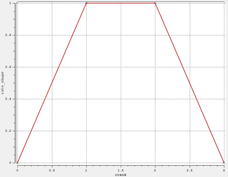
7.1.15. Instability models: Kelvin-Helmholtz (KH) model, Rayleigh-Taylor (RT) model, Discharge coefficient model
7.1.16. Injection temporal type: CYCLIC
7.1.17. Cyclic period: 720 deg.
7.1.18. Start of injection: -480 deg.
7.1.19. Injection duration: 191.2 deg.
7.1.20. Total injected mass:
The fuel flow rate is given as `dot(m)=7.5times10^-4 Kg//s`
Engine RPM `N=3000`rpm
Cyclic period: 720 deg. (2 revs. of crankshaft)
Time interval equivalent to 2 crankshaft revolutions (720 deg.), `Deltat`= (Number of revolutions)X60/(Engine RPM)=`(2times60)/3000=0.04s`
Mass of fuel injected within this time interval `m=dot(m)timesDeltat=7.5times10^-4Kg//stimes0.04s=3times10^-5Kg`
Hence total injected mass=`3times10^-5Kg`
7.1.21. Total number of injected parcels (per nozzle): 50000
7.1.22. Injection drop distribution: Predefined, Blob (specified nozzle diameter)
7.1.23. Temperature: 330K
7.1.24. Injection spray type: Solid cone spray
7.1.25. Nozzle diameter (for all four nozzles): 0.00025m
7.1.26. Circular injection radius (for all four nozzles): 0.000125m
7.1.27. Spray cone angle (for all four nozzles): 10 deg.
7.1.28. Location and orientation of nozzles:
Nozzle 0
center 0.0823357 0.00100001 0.07019
Align Vector -0.732501 0.210489 -0.647408
Nozzle 1
center 0.0823357 -0.00099999 0.07019
Align Vector -0.732501 -0.210489 -0.647408
Nozzle 2
center 0.0823357 -0.0004 0.07019
Align Vector -0.5 -0.2 -0.647408
Nozzle 3
center 0.0823357 0.0003 0.07019
Align Vector -0.5 0.2 -0.647408
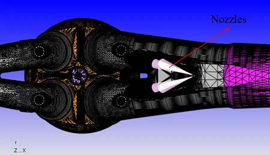
7.2. Combustion modeling
SAGE combustion model is used with the following settings:
Fuel species name: Iso-octane
Temporal type: CYCLIC
Cyclic period: 720 deg.
Start time: -17 deg.
End time: 130 deg.
Regions: Not region-dependent
Combustion temperature cutoff: 600K
Minimum HC species mole fraction: 1e-10
Adaptive zoning: Enabled
Temperature bin size: 5K
Reaction ratio bin size: 0.05
7.3. Turbulence modeling
RNG `K-epsilon` model is used to capture turbulence.
7.4. Source/sink modeling
The spark plug is modeled using two energy sources. These energy sources appear as source terms in the energy equation. This increases the temperature which in turn affects the chemical kinetics. Consequently more combustion species are generated and more heat is liberated. This heat again appears as a source term in the energy equation and results in temperature rise. In this way the combustion process continues.
The spark plug energy profile, applied for simulation, is given below:
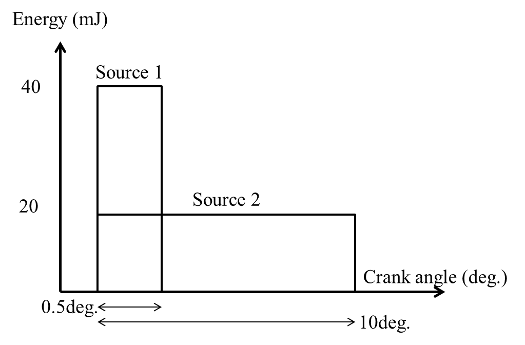
The following settings are used for the two energy source:
Source 1:
Source: Energy
Source units: Energy
Value: 20mJ
Maximum temperature: 50000K
Mode: CYCLIC
Start time: -15 deg.
End time: -14.5 deg.
Period: 720 deg.
Shape type: Sphere
Center of the sphere (x,y,z): -0.003 0.0 0.0091 (m)
Sphere radius (m): 0.0005
Source 2:
Source: Energy
Source units: Energy
Value: 20mJ
Maximum temperature: 50000K
Mode: CYCLIC
Start time: -15 deg.
End time: -5 deg.
Period: 720 deg.
Shape type: Sphere
Center of the sphere (x,y,z): -0.003 0.0 0.0091 (m)
Sphere radius (m): 0.0005
8. Grid Control
8.1. Base grid
dx=dy=dz=0.004m
8.2. Adaptive Mesh Refinement
The following settings are used for AMR:
AMR Group 1: Velocity
Minimum cells: 1
Maximum cells: 2000000
Regions: Cylinder, Intake system and Intake system2
Embed type: Sub-Grid Scale (SGS)
Timing control type: PERMANENT
Maximum embedding level: 3
Minimum grid size: (Base grid size)/2^(Embedding level)=(Base grid size)/2^3=(Base grid size)/8=0.0005m
Sub-Grid criterion: 1m/s
Use AMR when parcel count exceeds: 50
AMR Group 2: Temperature
Minimum cells: 1
Maximum cells: 2000000
Regions: Cylinder, Intake system and Intake system2
Embed type: Sub-Grid Scale (SGS)
Timing control type: CYCLIC
Start: -17 deg.
End: 135 deg.
Cycle period: 720 deg.
Maximum embedding level: 3
Minimum grid size: (Base grid size)/2^(Embedding level)=(Base grid size)/2^3=(Base grid size)/8=0.0005m
Sub-Grid criterion: 2.5K
8.3. Fixed embedding
Fixed embedding is applied at specific locations as follows:
i. Embedding 1:
Type: BOUNDARY
Boundary: Intake_Valve_Angle
Mode: PERMANENT
Scale: 3
Embed Layers: 1
Resultant grid size: (Base grid size)/2^(Embed scale)=(Base grid size)/2^3=(Base grid size)/8=0.0005m
ii. Embedding 2:
Type: BOUNDARY
Boundary: Exhaust_Valve_Angle
Mode: PERMANENT
Scale: 3
Embed Layers: 1
Resultant grid size: (Base grid size)/2^(Embed scale)=(Base grid size)/2^3=(Base grid size)/8=0.0005m
iii. Embedding 3:
Type: CYLINDER
Mode: PERMANENT
Scale: 1
Resultant grid size: (Base grid size)/2^(Embed scale)=(Base grid size)/2^1=(Base grid size)/2=0.002m
The centers of a cylinder:
x=0, y=0, z=0.08m
x=0, y=0, z=-0.15m
Cylinder radius 1: 0.05m
Cylinder radius 2: 0.05m
iv. Embedding 4:
Type: CYLINDER
Mode: PERMANENT
Scale: 2
Resultant grid size: (Base grid size)/2^(Embed scale)=(Base grid size)/2^2=(Base grid size)/4=0.001m
The centers of a cylinder:
x=0, y=0, z=0.018m
x=0, y=0, z=-0.15m
Cylinder radius 1: 0.05m
Cylinder radius 2: 0.05m
v. Embedding 5:
In order to avoid numerical diffusion of the energy supplied by the two energy sources (created to mimic the spark ignition process), the grid near them must be refined. Hence two spherical type fixed embedding zones, Embedding 5 and Embedding 6, are created at the spark location with the following settings:
Entity type: Sphere
Mode: CYCLIC
Period: 720 deg.
Scale: 5
Resultant grid size: (Base grid size)/2^(Embed scale)=(Base grid size)/2^5=(Base grid size)/32=0.000125m
Start time: -16 deg.
End time: 7 deg.
Center of the sphere (x,y,z): -0.003 0.0 0.0091 (m) (Same as the spark location)
Radius: 0.001m
vi. Embedding 6:
Entity type: Sphere
Mode: CYCLIC
Period: 720 deg.
Scale: 3
Resultant grid size: (Base grid size)/2^(Embed scale)=(Base grid size)/2^3=(Base grid size)/8=0.0005m
Start time: -16 deg.
End time: 7 deg.
Center of the sphere (x,y,z): -0.003 0.0 0.0091 (m) (Same as the spark location)
Radius: 0.003m
vii. Embedding 7:
Entity type: INJECTOR
Mode: CYCLIC
Period: 720 deg.
Scale: 4
Resultant grid size: (Base grid size)/2^(Embed scale)=(Base grid size)/2^4=(Base grid size)/16=0.00025m
Start time: -482 deg.
End time: -286 deg.
Radius 1: 0.002m
Radius 2: 0.004m
Length: 0.02m
V. Results
1. Cylinder volume
As a result of the reciprocating piston motion, the cylinder volume oscillates between a maximum value and a minimum value. The ratio of the maximum cylinder volume (when the piston is at the BDC (Bottom Dead Center)) to the minimum cylinder volume (when the piston is at the TDC (Top Dead Center)) is known as compression ratio. The figure attached below shows the cylinder volume as a function of crank angle.
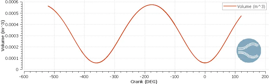
Maximum cylinder volume: `V_1=5.742195times10^-4m^3`
Minimum cylinder volume: `V_2=5.7029438times10^-5m^3`
Compression ratio: `r_c=V_1/V_2=10.07` (Typical of SI engines)
2. Cylinder pressure
The cylinder pressure rises during the compression stroke and as the combustion process begins the rate of pressure rise becomes even steeper and the cylinder pressure finally peaks. The cylinder pressure then falls during the expansion stroke. The figure attached below shows the cylinder pressure as a function of crank angle (popularly known as p-theta diagram).
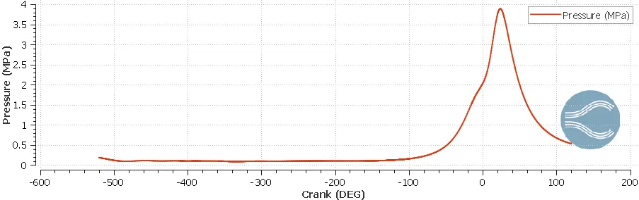
The plot agrees quite well with the characteristic p-theta diagram of SI engines. The peak pressure in the cylinder is 3.89MPa.
3. Mean temperature
The figure attached below shows the mean (volume-averaged) temperature within the cylinder as a function of crank angle.
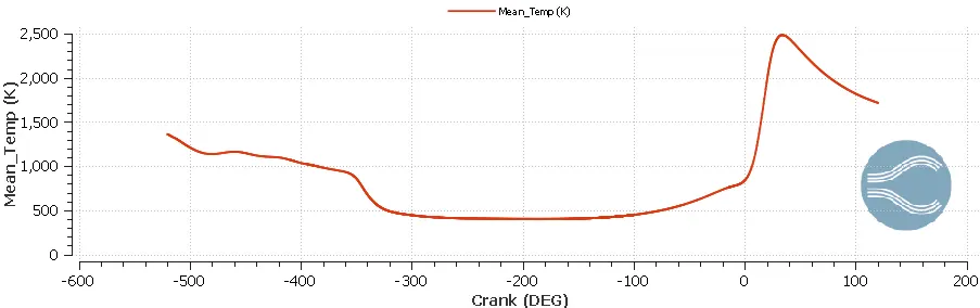
The peak in mean temperature can be attributed to the temperature rise due to combustion. Also it can be seen that the mean temperature peak and pressure peak occur at nearly the same value of crank angle. The peak mean temperature in the cylinder is 2483.18K.
This kind of data is very useful if one is interested in performing thermal analysis of the engine structure, as it requires the gas-side boundary conditions. For this purpose the entire profile (shown in the plot) can be used. It should be emphasized here that the wall temperature values can't be obtained from a CFD simulation (such as the present one) without using a wall heat transfer model. This is because a CFD simulation can only predict temperature field in the gas phase. The problem of heat transfer between the gas phase and the engine wall still remains unsolved. Hence a suitable wall heat transfer model is required.
4. Trapped mass in the cylinder
The figure attached below shows the trapped mass in the cylinder as a function of crank angle.
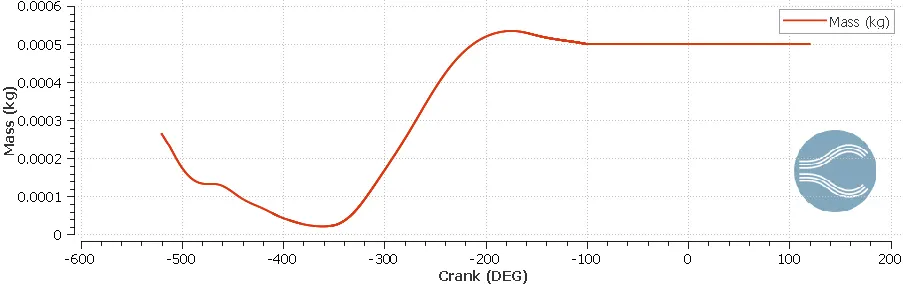
The mass inside the cylinder decreases during the exhaust stroke and eventually reaches a minimum value. This value is useful as it quantifies the mass of species in the cylinder after the exhaust stroke. It may be due to the presence of unburnt fuel or combustion products in the cylinder. This mass should be as small as possible for the engine to achieve its maximum power output. The plot shows that for the present engine the trapped mass is equal to `2.0996855times10^-5 Kg`.
5. Heat Release Rate and Integrated Heat Release
The figure attached below shows the heat release rate as a function of crank angle.
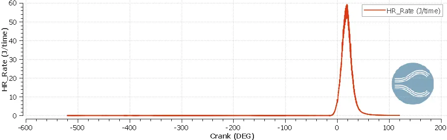
Heat release rate signifies the amount ofheat released per unit time (crank angle in the present case) in the combustion process. According to the plot, the peak heat release rate is approximately 60J/crank angle. Even more significant is the integrated heat release which quantifies the total energy released during the combustion process. The figure attached below shows the integrated heat release as a function of crank angle.
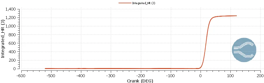
According to the plot, the value of integrated heat release is 1241.1646J. The integrated heat release can be used to calculate the combustion efficiency of the engine. Combustion efficiency denotes the ability of an engine to convert the energy content of the fuel into heat. Hence:
`eta_(combustion)=`(Integrated Heat Release)/(Energy content of the fuel)
For gasoline LHV (Lower Heating Value)=43.4MJ/Kg
Mass of gasoline fuel injected=`3times10^-5 Kg`
Energy content of the fuel=`3times10^-5 Kg times 43.4MJ//Kg=1302J`
Therefore `eta_(combustion)=(1241.1646J)/(1302J)=0.9533`
The combustion efficiency of the present engine is 95.33%. In other words, 95.33% of energy content in the fuel is released as heat during the combustion process in the present engine.
6. Liquid spray drops
The figure attached below shows the number of liquid parcels in the Cylinder region as a function of crank angle.
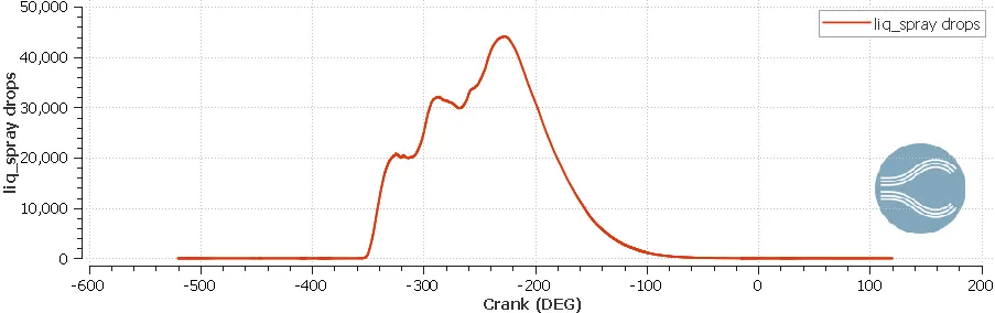
It is evident from the plot that the maximum number of parcels present in the Cylinder region is: 45000 (approximately). The number of liquid parcels in the Cylinder region decrease after some time due to evaporation and combustion. Eventually the number of liquid parcels in the Cylinder region drop down to zero, which indicates that there is no liquid fuel present in the system. In other words, the combustion process leaves no unburnt fuel in the system.
The figure attached below shows the mass of liquid fuel (iso-octane) present in the Cylinder region as a function of crank angle.
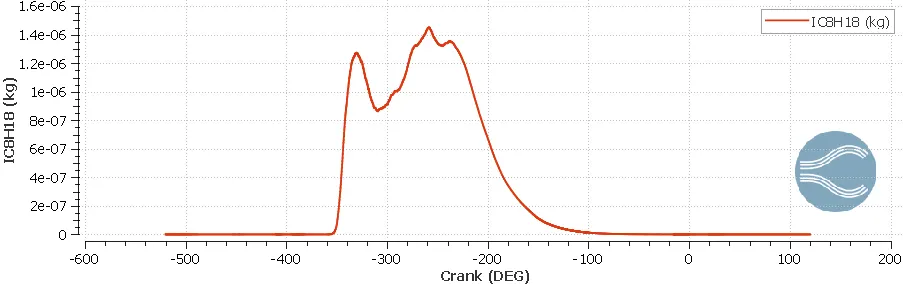
The plot shows a similar trend as the number of liquid parcels. At a certain crank angle, the mass of liquid fuel reaches a maximum value and subsequntly it decreases due to evaporation and combustion. Ultimately there is no liquid fuel left in the system, which indicates that the combustionprocess leavesno unburnt fuel.
The figure attached below shows the number of liquid parcels in the Intake system2 region as a function of crank angle.
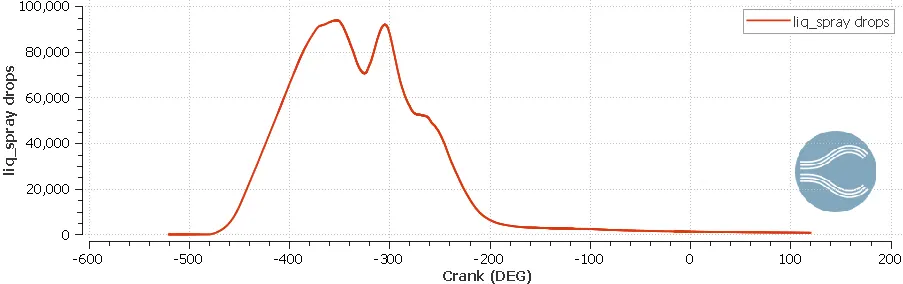
According to the plot the maximum number of liquid parcels in the Intake system2 region is: 95000 (approximately). Over time, the number of liquid parcels decrease as they enter into the Cylinder region. However unlike the Cylinder region, the number of liquid parcels in the Intake system2 region never drop down to zero. This indicates that there is always some amount of liquid fuel remaining in the intake port. A similar trend is shown by the mass of liquid fuel present in the Intake system2 region.
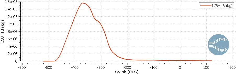
The plot shows that the mass of liquid fuel (iso-octane) remaining in the intake port is equal to: `9.1386068times10^-8 Kg`. This quantity should be as small as possible relative to the total amount of liquid fuel injected. For the present engine this value is equal to `3times10^-5 Kg`. Hence the liquid fuel remaining in the intake port is only 0.3% of the total liquid fuel injected which is indeed quite small.
7. Emissions
The figure attached below shows the mass of combustion products (emissions), generated in the Cylinder region as a result of combustion chemical reactions, as a function of crank angle.
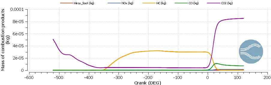
The mass of different combustion products generated in the Cylinder region are as follows:
i. Hiroy Soot: `2.5303679times10^-8 Kg`
ii. `NO_x`: `1.2864612times10^-6 Kg`
iii. HC: `1.440608times10^-8 Kg`
iv. CO: `7.1112219times10^-6 Kg`
v. `CO_2`: `8.5066703times10^-5 Kg`
Emission characteristics play a very crucial role in engine design. A well designed engine should have very low emissions. In other words the mass of combustion products released by the engine into the environment should be very small.
8. Engine Power and Engine Torque
Engine power and engine torque are very important performance parameters for IC engines. An IC engine operates on thermodynamic cycle and convert heat released during combustion into expansion work. This work can be calculated by estimating the area under the curve of a PV diagram. The figure attached below shows the PV diagram for the Cylinder region.
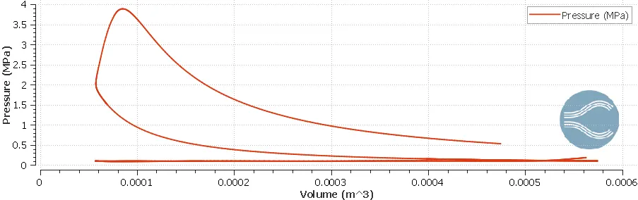
For estimating the work delivered by an IC engine, CONVERGE provides a convenient tool known as Engine Performance Calculator. All details relevant to the engine are fed into the tool and it generates importance performance parameters for the engine. Given below are the engine performance parameters generated by the tool for the present engine:
i. Work: 468.646N-m
ii. Indicated Mean Effective Pressure (IMEP): 0.8964280MPa
iii. CA10: 6.837170 deg.. It denotes the crank angle at which 10% combustion is finished (10% of the fuel is burnt).
iv. CA50: 18.4623 deg.. It denotes the crank angle at which 50% combustion is finished (50% of the fuel is burnt).
v. CA90: 31.701 deg.. It denotes the crank angle at which 90% combustion is finished (90% of the fuel is burnt).
vi. Peak Firing Pressure (PFP): 3.888840MPa
vii. Heat Release Rate Peak: 59.35620J/deg.
Calculation of Engine Power:
Since the engine under consideration is a four-stroke engine, it delivers work/power once in every two revolutions. Hence if the engine RPM is 3000 then in one minute it delivers work/power 1500 times. In other words in one minute, the engine delivers `468.646times1500J`. Therefore in one second the engine delivers `(468.646times1500)/60 J` which is nothing but indicated power of the engine. Hence:
Indicated Power of the engine=`(468.646times1500)/60 W=11716.15W=11.716KW`
If the frictional losses are neglected in the present analysis then the brake power is same as the indicated power. Therefore:
`P=(2piNT)/60`
Hence Engine Torque: `T=(Ptimes60)/(2piN)=(11716.15times60)/(2pitimes3000) N-m=37.294N-m`
9. Animations
9.1. Temperature contours
The animation shows the temperature contours plotted over a sectional plane passing through the engine as a function of time. The four strokes namely intake stroke, compression stroke, expansion stroke and exhaust stroke are clearly visible in the animation. Also the combustion process including the spark ignition and flame propagation are also evident in the animation.
9.2. Parcel temperature contours
The animation shows the parcel temperature contours as a function of time. The parcel spray into the intake port, the movement of parcels through the intake valves into the cylinder and their motion inside the cylinder can be easiliy observed in the animation.
VI. Conclusion:
Full hydrodynamic simulation is performed on a given port fuel injected engine geometry. Engine performance, combustion characteristics and emission characteristics are studied through simulation results. The following conclusions can be made from the study:
i. The compression ratio for the engine is 10.07 which agrees well with SI engines.
ii. The peak pressure inside the cylinder is 3.888840MPa.
iii. The peak mean temperature in the cylinder is 2483.18K.
iv. The trapped mass inside the cylinder is `2.0996855times10^-5 Kg`.
v. Peak Heat Release Rate is 59.35620J/deg.
vi. Integrated Heat Release is 1241.1646J
vii. Combustion efficiency of the engine is 95.33%.
viii. No liquid spray is left in the cylinder after combustion.
ix. The amount of liquid fuel in the intake port is `9.1386068times10^-8 Kg`.
x. Mass of Hiroy Soot in the cylinder: `2.5303679times10^-8 Kg`
xi. Mass of `NO_x` in the cylinder: `1.2864612times10^-6 Kg`
xii. Mass of HC in the cylinder: `1.440608times10^-8 Kg`
xiii. Mass of CO in the cylinder: `7.1112219times10^-6 Kg`
xiv. Mass of `CO_2` in the cylinder: `8.5066703times10^-5 Kg`
xv. Power delivered by the engine: 204.485W
xvi. Engine Torque: 0.6509N-m