Week 10: Project 1 - FULL HYDRO case set up (PFI)
AIM: To perform combustion for the given PFI with the given details and study the charactersitics of the process by post processing the results.
What is Combustion?
Combustion, or burning, is a high-temperature exothermic redox chemical reaction between a fuel (the reductant) and an oxidant, usually atmospheric oxygen, that produces oxidized, often gaseous products, in a mixture termed as smoke. Combustion does not always result in fire, but when it does, a flame is a characteristic indicator of the reaction. While the activation energy must be overcome to initiate combustion (e.g., using a lit match to light a fire), the heat from a flame may provide enough energy to make the reaction self-sustaining.
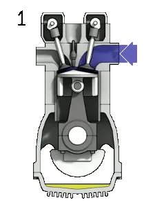
A four-stroke (also four-cycle) engine is an internal combustion (IC) engine in which the piston completes four separate strokes while turning the crankshaft. A stroke refers to the full travel of the piston along the cylinder, in either direction. The four separate strokes are termed:
- Intake: Also known as induction or suction. This stroke of the piston begins at top dead center (T.D.C.) and ends at bottom dead center (B.D.C.). In this stroke the intake valve must be in the open position while the piston pulls an air-fuel mixture into the cylinder by producing vacuum pressure into the cylinder through its downward motion. The piston is moving down as air is being sucked in by the downward motion against the piston.
- Compression: This stroke begins at B.D.C, or just at the end of the suction stroke, and ends at T.D.C. In this stroke the piston compresses the air-fuel mixture in preparation for ignition during the power stroke (below). Both the intake and exhaust valves are closed during this stage.
- Combustion: Also known as power or ignition. This is the start of the second revolution of the four stroke cycle. At this point the crankshaft has completed a full 360 degree revolution. While the piston is at T.D.C. (the end of the compression stroke) the compressed air-fuel mixture is ignited by a spark plug (in a gasoline engine) or by heat generated by high compression (diesel engines), forcefully returning the piston to B.D.C. This stroke produces mechanical work from the engine to turn the crankshaft.
- Exhaust: Also known as outlet. During the exhaust stroke, the piston, once again, returns from B.D.C. to T.D.C. while the exhaust valve is open. This action expels the spent air-fuel mixture through the exhaust valve
STEPWISE PROCEDURE FOR FLAGGING THE PORT FUEL INJECTOR:
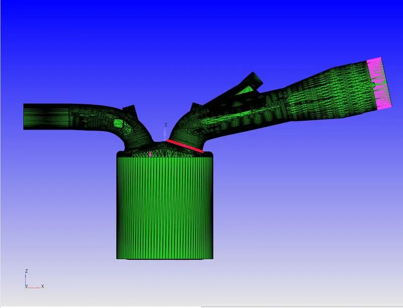
Above is the Port fuel injector. The most basic step prior to flagging is to run a diagnostic test on the imported geometry to ensure that the geometry is complete and errors are non-existant.
A diagnostic test was run on this geometry and the following were determined.
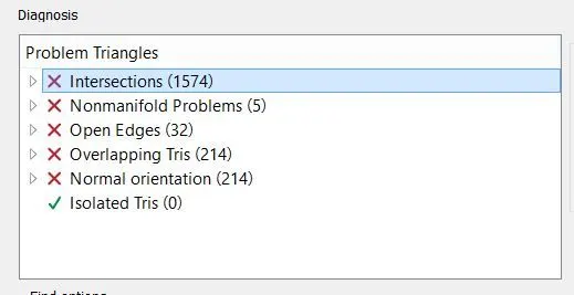
The above shows the errors we face when the diagonosis was done. Now these issues are solved simultaneously while flaging the geometry. Initially we flag the liner, cylinder head and piston by creating a fence to ensure that the flaging is done correctly.
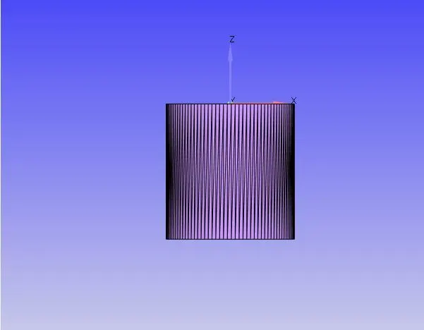
Liner:
Piston:
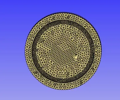
Initially, there were issues such as open edges in the piston region which was sorted using the patch tool.
Cylinder Head:
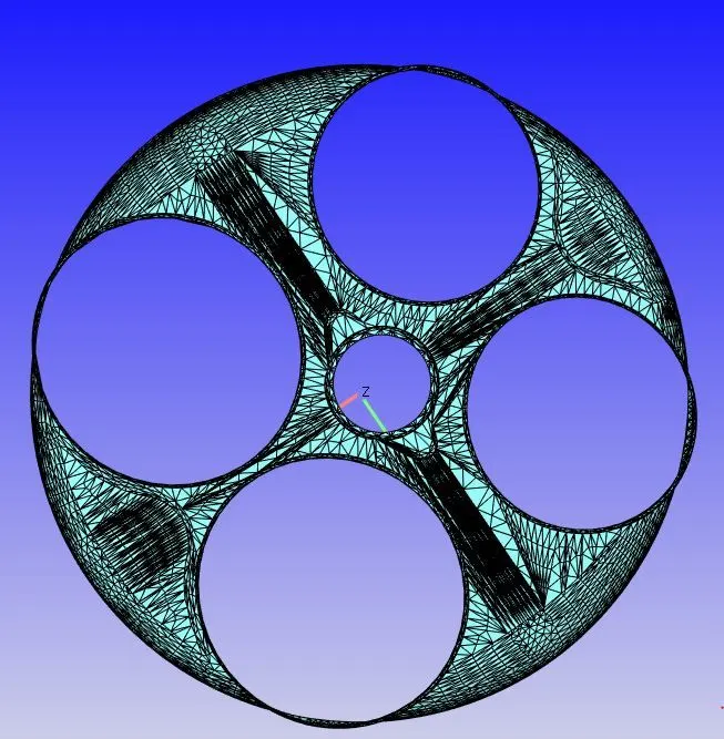
Exhaust port:
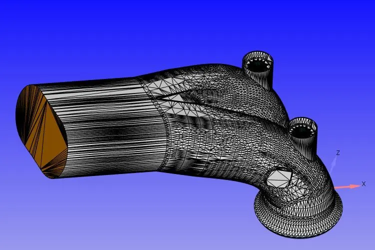
Intake port:
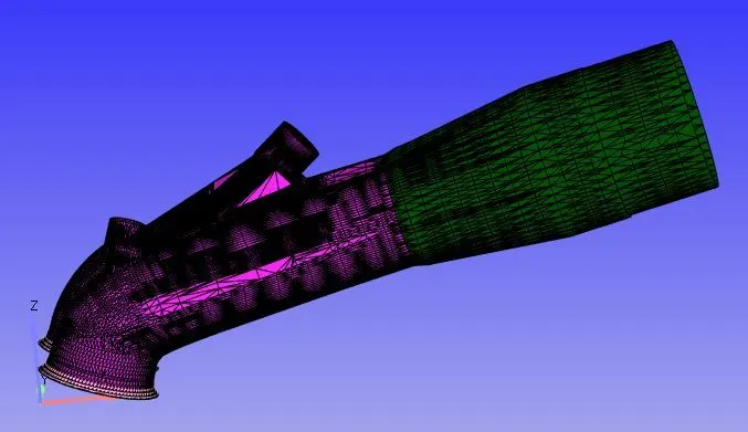
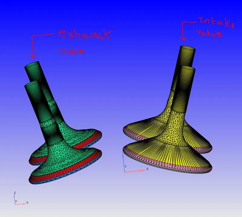
Intake and Exhaust valves:
Spark plug:
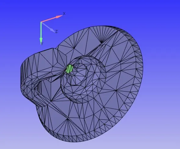
In this case we flage the spark plug and terminal differently in spite of them being the same component. This is done because the terminal is at a higher temperature than the spark plug in order to generate a spark.
Totally flaged surface:
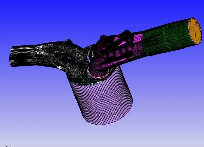
The PFI grouped by regions:
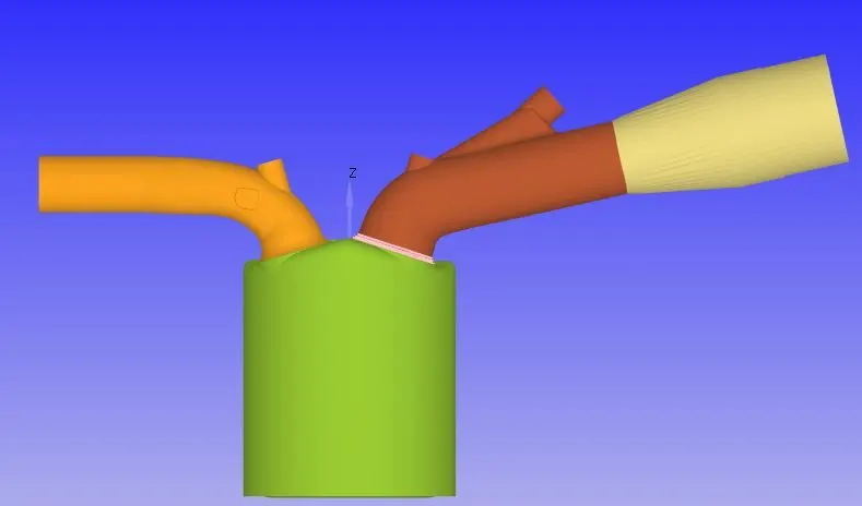
In the setup, four regions were created. This was because, the parts of the PFI generally are at varying temperatures.
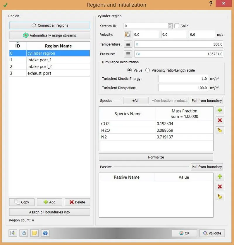
Below is the list of flagged parts:
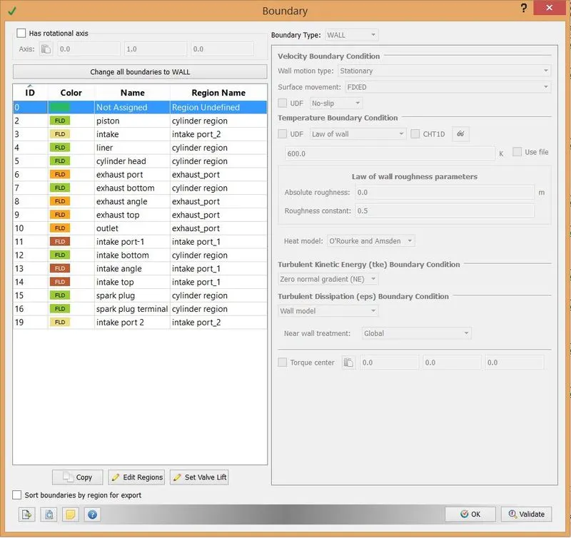
Brief Procedure:
- Here crank angle based IC engine was selected as the application.
- Here, we opt for solid and gas simulation.
- In the simulation parameters, we select the transient solver, crank angle based engine simulation and make sure that the mode of simulation is no hydrodynamic.
- We setup the boundaries as required also we assign the region to each of the boundary.
- In this case, we assign 4 regions. This is because we are dealing with locations with varying temperatures.
- Here we employ the turbulence modeling where we use the RANS method and we use the RNG k ε.
- The most important aspect in this model is to make sure that the model is dimentioned in meters. Also the base grid dimensions are to be mentioned in meters.
- The post processing is done on the results once the simulation is complete.
Post processing output:
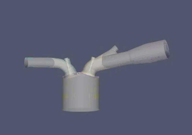
Mesh:
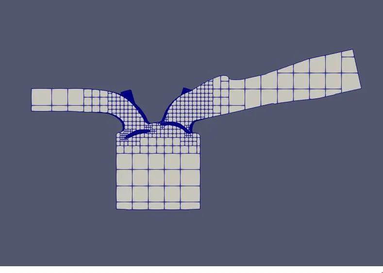
SETTING UP THE HYDRO CASE:
The following inputs are given in order to provide the software with the specifics of the engine.
Engine Geometric Parameters
- Bore =0.086 m
- Stroke = 0.09 m
- Connecting rod length = 0.18 m
- RPM = 3000
Run parameters
- Simulation mode: Hydro
Simulation time parameters
- Start time : -520 deg
- end time : 120 deg
Boundary conditions
- Piston temperature - 450K
- Liner temperature - 450K
- Head temperature - 450K
- Spark Plug temperature - 550K
- Spark Plug electrode temperature - 600K
- Exhaust ports temperature - 500K
- Exhaut outflow - 1 bar
- Exhaust outlflow temperature - 800k
- Exhaust species concentration - Calculate the stoichiometric condition
- Exhaust valve top temperature - 525K
- Exhaust valve angle temperature - 525K
- Exhaust valve bottom temeprature - 525K
- Intake port - 1 temperature 425K
- Intake port - 2 temperature 425K
- Inflow pressure - 1 bar total pressure
- Inflow temperature - 363K
- Inflow species - Air
- Intake valve top temperature - 480K
- Intake valve angle temperature - 480K
- Intake valve bottom temeprature - 480K
Initial conditions
- Intake port - 1 (closer to combustion chamber)
- ic8h18 - 0.025508
- o2 - 0.20157
- n2 - 0.77292
- Temperature - 390k
- pressure - 1 bar
- Intake port - 2 (away from combustion chamber)
- Air
- Temperature - 370K
- Pressure - 1 bar
- Cylinder
- Pressure - 1.85731 bar
- Temperature - 1360K
- Stoichiometric composition
Injection Parameters
- Fuel flow rate = 7.5e-4 Kg/second
- Injection start time = -480.0
- Injection duration = 191.2
- Fuel temperature = 330K
Nozzle positions
Nozzle diameter = 250 micro-meter
Circular injection radius = Nozzle radius
Spray cone angle = 10
- Nozzle 0
- center 0.0823357 0.00100001 0.07019
- Align Vector -0.732501 0.210489 -0.647408
- Nozzle 1
- center 0.0823357 -0.00099999 0.07019
- Align Vector -0.732501 -0.210489 -0.647408
- Nozzle 2
- center 0.0823357 -0.0004 0.07019
- Align Vector -0.5 -0.2 -0.647408
- Nozzle 3
- center 0.0823357 0.0003 0.07019
- Align Vector -0.5 0.2 -0.647408
Spark Ignition Parameters
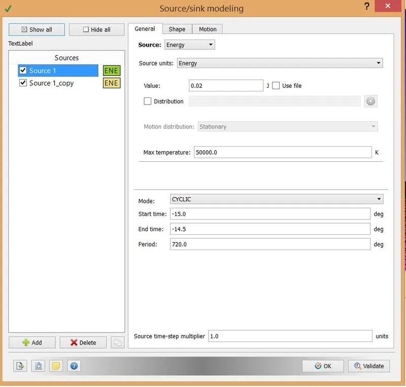
- Start of spark = -15 deg
- Spark duration = 10 deg
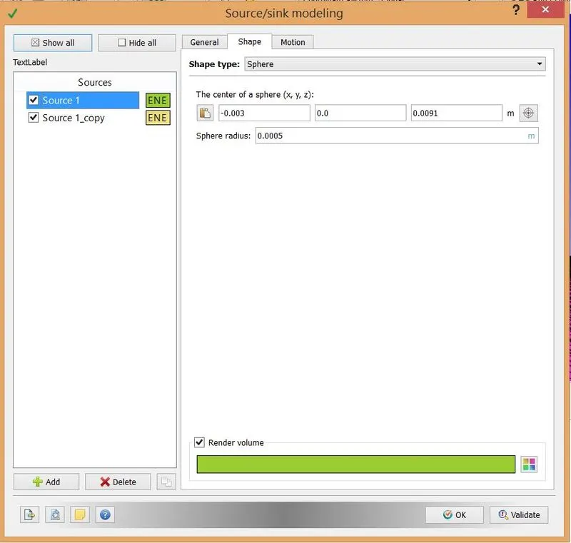
- Spark location = -0.003 0 0.0091
- Spark radius = 0.0005m
Note: Most of the setup was done while flagging the boundary and running a no hydro simulation
However, the procedure to setup the combustion model and spray model is given below.
Setting up the combustion model:
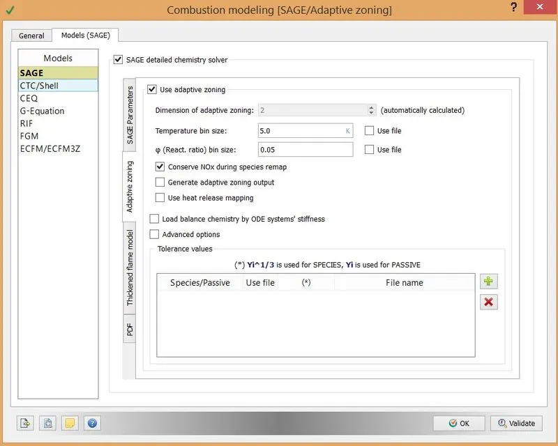
- In this module we opt for the SAGE model. This is because of its robustness and its ability to produce results nearly equal to the actual values .
- In the general section the basic start and end times are given as input. Here the time is mentioned in degrees as we are simulating a reciprocating IC engine in which we predict the time of motion of moving parts in degrees due to the rotary motion of the camshaft.
Step 1:
Step 2:
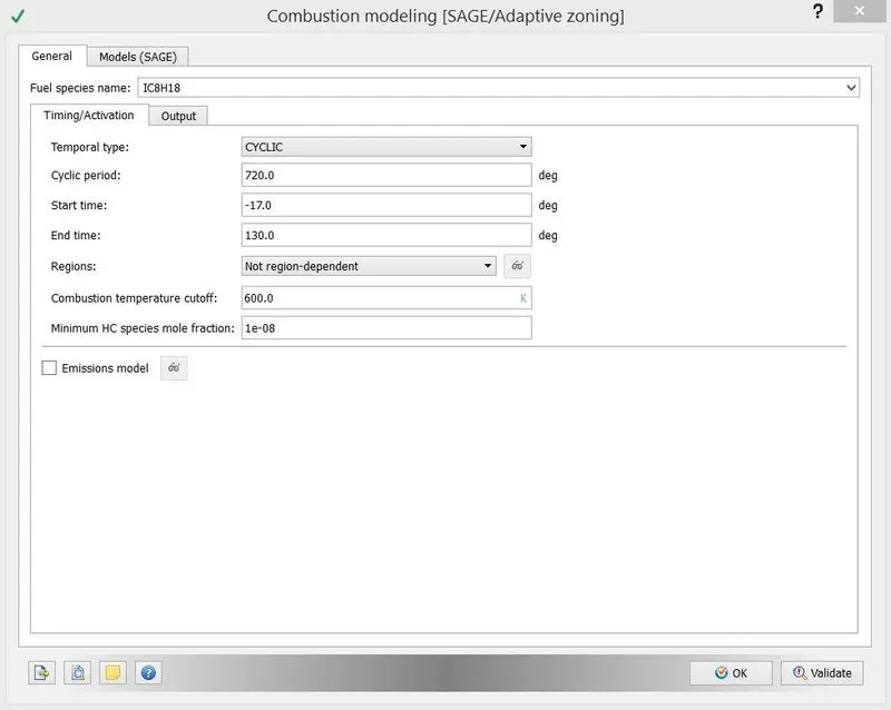
Setting up the Spray model:
- Initially the parcel distribution type was selected. In this case the distribute parcels evenly throughout the cone was selected to ensure that the parcels are sprayed in a even fashion.
- The turbulence model opted was O'Rouke since this model is known for capturing turbulence very well.
- The evapouration model was checked and for the source the second option was opted.
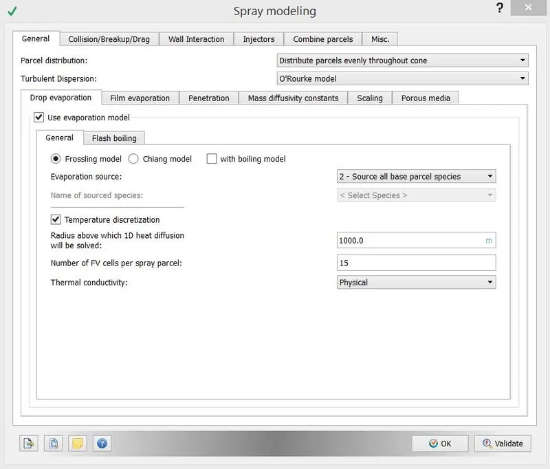
- The most quintessential step is to setup the injectors.
- Here we setup a injector in the injector tab.
- In order to setup the spray pattern the injectors properties were edited as per requirement.
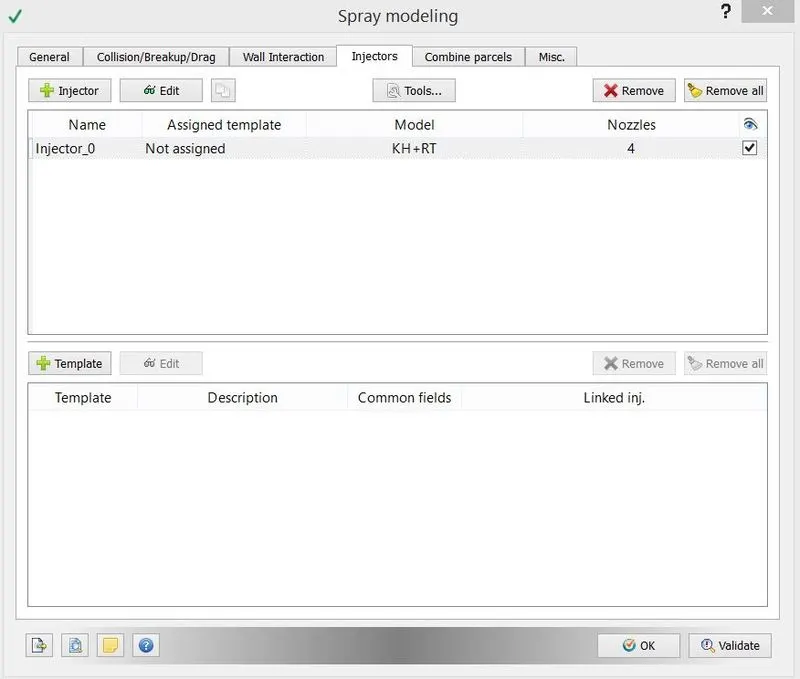
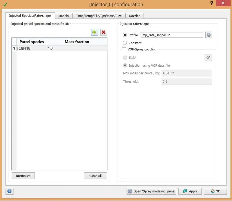
- The profile of the spray was inputed by editing the injectors property as shown below.
- The following profile was created.
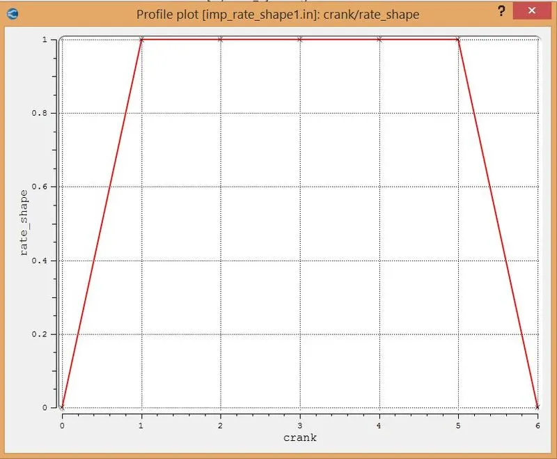
- The model selected were the KH and RT models which ensure better results.
- The number of nozzles were inputed in the nozzle section as shown below:
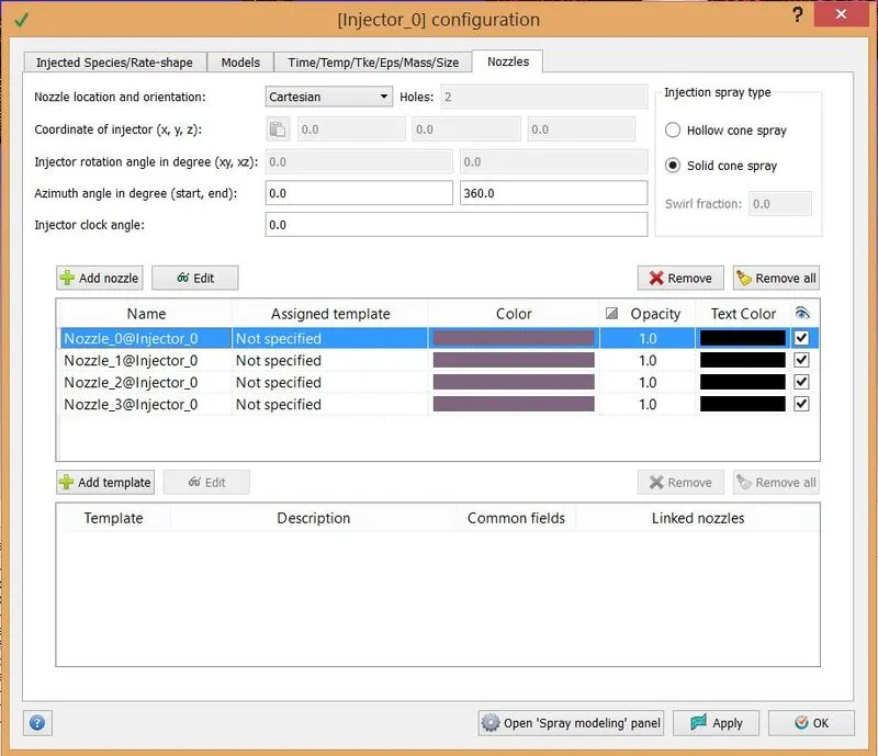
- The orientation of the nozzles were as per the cartesian coordinates.
- In order to specify the location and the basic inputs of the nozzles, the entries were edited and the locations were specified as mentioned in the information provided above in this report.
- This completes the spray modeling.
- The end result is as shown below:
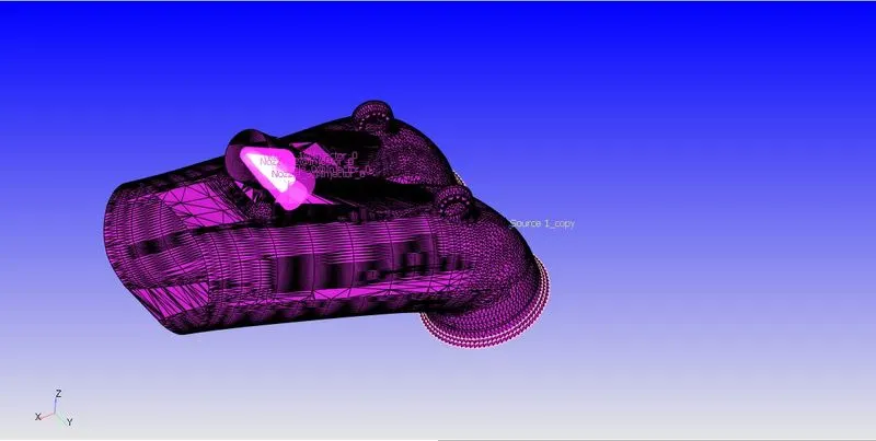
A clearer image of the nozzles:

Setting up the Source model for the spark plug:
- The spark plug is usually at a higher temperature compared to the rest of the parts.
- Also it is the source for igniting the fuel and air mixure.
- Thus a source model was initialized as per requirement which is shown in the below images:
COMPRESSION RATIO:
The compression ratio (CR) is defined as the ratio of the volume of the cylinder and its head space (including the pre-combustion chamber, if present) when the piston is at the bottom of its stroke to the volume of the head space when the piston is at the top of its travel (‘top dead centre’, tdc). Typically, petrol engines have a CR of 8–10, while diesel engines have a CR of 15–20. The CR of petrol engines is limited by the requirement that the fuel burns uniformly in the cylinder and does not ignite thermally prior to the spark (so-called ‘engine knocking’). In a spark-ignition engine, the CR at which pre-ignition takes place is determined by the octane number of the petrol. High-octane fuel permits a high CR.
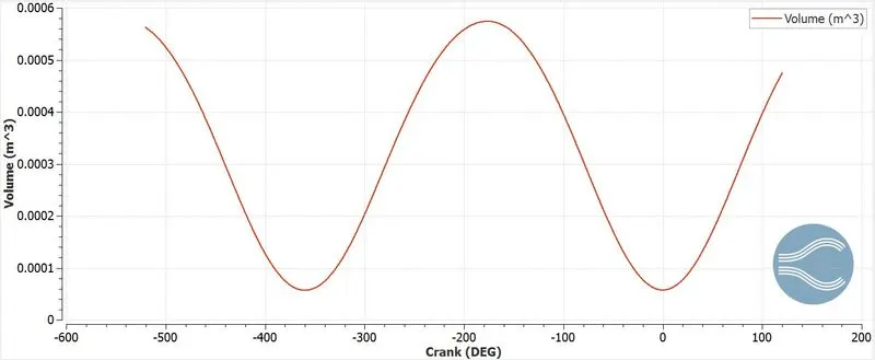
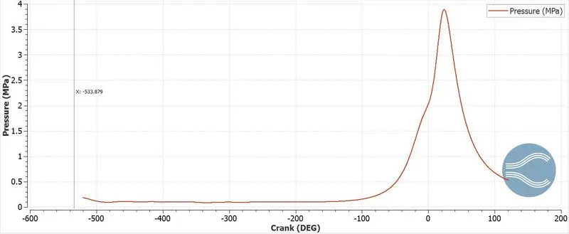
Above is the plot of pressure variation in the cylinder region.
We find the maximum and minimum values of volumes from the plot data. The maximum and minimum values are listed below:
MAXIMUM VALUE:

MINIMUM VALUE:

The compression ratio for this model was found to be:
CR=0.0005742195/5.7539186e-5
CR=9.98
So the compression ratio was found to be 9.98:1, nearly 10:1
Need a wall heat transfer model and why can't we predict the wall temperature from the CFD simulation?
CFD models usually predict the temperature a fluid and the equations are ment for the same. The Navier Stroke equation is strictly used to find solution to fluid problems. Usually the solver assumes the walls as a void while calculating the solution. This essentially means that the heat transfer caused due to convection and condution to the liner and the engine block is essentially ignored. In real life scenarios, we need to consider the losses to the other parts of the arrangement inorder to ensure that the energy is being utilized to the fullest. In order to study heat transfer in solids we enable the conjugate heat transfer model.
COMBUSTION EFFICIENCY:
Combustion efficiency is the calculation / measurement, in percentage, of how well your equipment is burning a specific fuel. Complete combustion efficiency (100%) would extract all the energy available in the fuel. However, 100% combustion efficiency is not realistically achievable. Various combustion processes produce combustion efficiencies from 0% to 95+%. Combustion efficiency calculations assume complete fuel combustion and are based on three factors:
- The chemistry of the fuel.
- The net temperature of the stack gases
- The percentage of oxygen or CO2 by volume after combustion.
`eta_c = ("Heat released")/(m_f .Q_h)`
Heat released = enthalpy of reactants - enthalpy of products
This is obtained directly from the plot below:
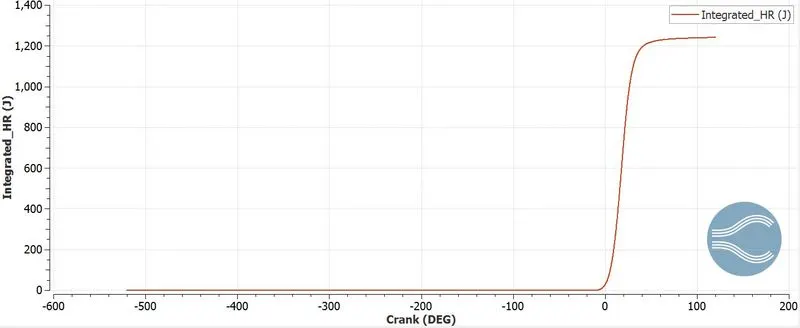
Heat released = 1241.1646 J
LHV of Iso octane= 44.65128315MJ/Kg
mass of fuel = 3e-5
`eta_c=1241.1646/(44.6512.10^6 . 3.10^-5)`= 92.65%
Power of the engine:
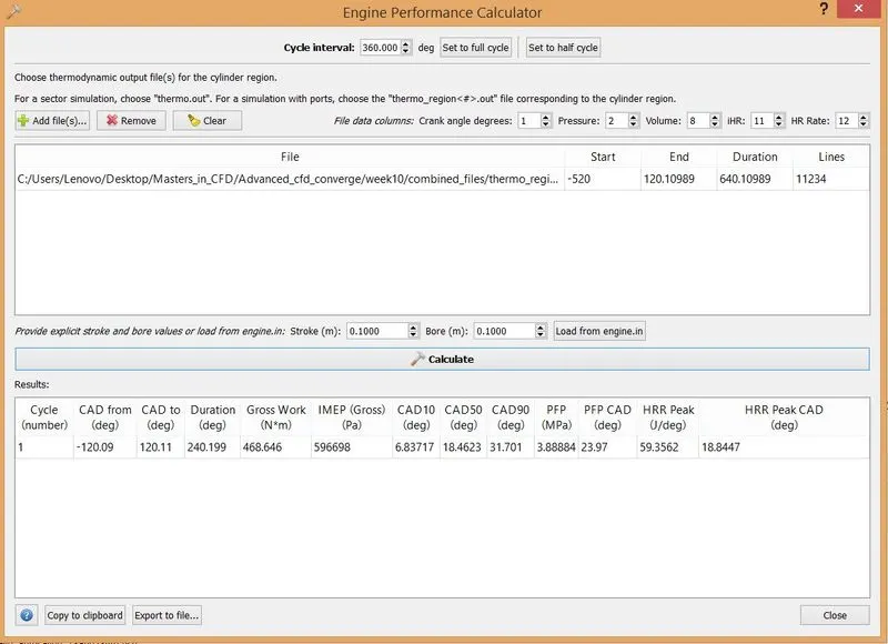
Converge has a tool known as the engine performance calculator through which the work of the engine is found.
In the case the work was found to be 468.646 Nm.
Now power is the ratio of work to time. In this case the time taken to complete the combustion was 240.199deg.
Engine RPM=3000
In RPS=50
In DPS =50 x 360=18000 dps
Time of combustion in seconds= 240.199/180000
Time of combustion in seconds=0.01334s
Power=work/time =468.646/0.01334=35130 j/s=35.130Kj/s
Since, Power(P) = (2*π*N*T)/60
`T=(60*P)/(2`pi`*N)`
T=111.8817Nm
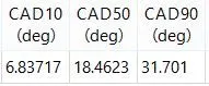
Significance of ca10, ca50 and ca90:
Ca10, Ca50 and Ca 90 represent the crank angle at which 10%,50% and 90% of fuel is burnt. These parameters can be found in the engine performance calulator.
Ca10: Denotes start of ignition
Ca50: Denotes phase change.
Ca90: Denotes end of combustion.
Combustion Chamber charactersitics:
Pressure:
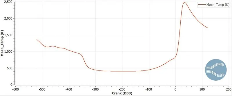
Temperature:
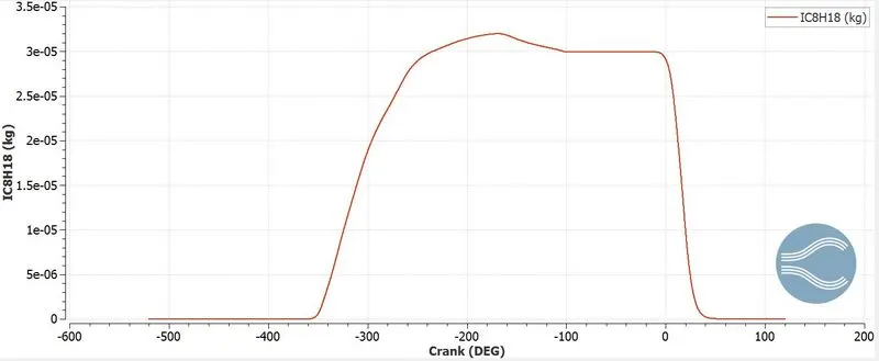
Mass of Fuel:
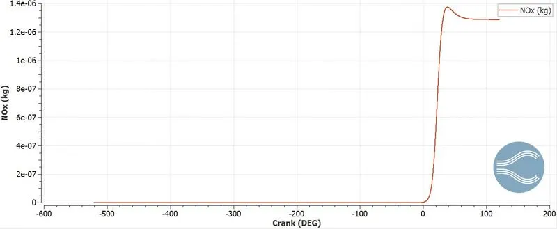
Exhaust emissions:
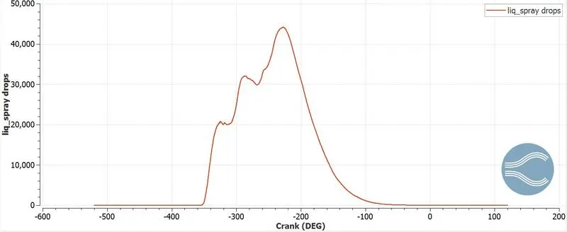
liquid spray plot:
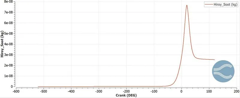
Hiroy Soot plot:
Links to animation:
Flame propogation:
Velocity:
PFI Animation: