Week 10: Modeling and Simulation of flow around an Ahmed Body

AIM:

• To use Converge CFD to model and simulate flow around an Ahmed Body and compare the simulation results to experimental data provided.

OBJECTIVE:

• Using any CAD package, create the CAD model.
• Setup a coarse CFD simulation
• Set up a virtual wind tunnel.
• Use the appropriate boundary conditions and solver settings.
• Display an animation of the velocity and pressure distributions on a cut plane.
• Allow wall-averaged outputs to be used to calculate drag and lift forces.

THEORY:

Ahmed's body:

• Ahmed's body is a generic car body that resembles all of the important flow features around a vehicle. S.R.Ahmed's experimental work was the first to define and characterise this generic form. This body enables us to capture all of the characteristics and features that are relevant to vehicle bodies. This body can be used for a variety of experiments, such as calculating drag and lift, which are important in the design of car bodies today. This can also be used to capture wake regions, flow separation, vortices, and so on. Different slant angles produce different values for the drag coefficient.

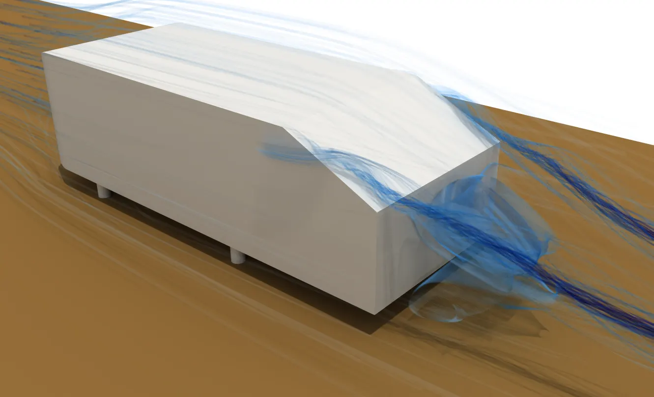
Three main features of Ahmed's body were seen in the wake:

1. The A recirculation region formed as the flow separates at the top of the model's vertical back surface.

2. The separation at the model's base creates the B recirculation region.

3. C-pillar vortices form as vorticity in the side boundary layers rolls up and over the slant edges.

• The wake was found to be extremely sensitive to slant angle. The flow remains attached over the slant for slant angles less than 12°. The flow is primarily two-dimensional and has little drag. As the c-pillar vortices form between 12° and 30°, the flow becomes much more three-dimensional. At 30°, these reach their peak strength. As the low-pressure cores act on the rear surfaces, the drag increases significantly. After 30°, the flow completely separates from the slant. This causes a sharp drop in drag and weaker c-pillar vortices.

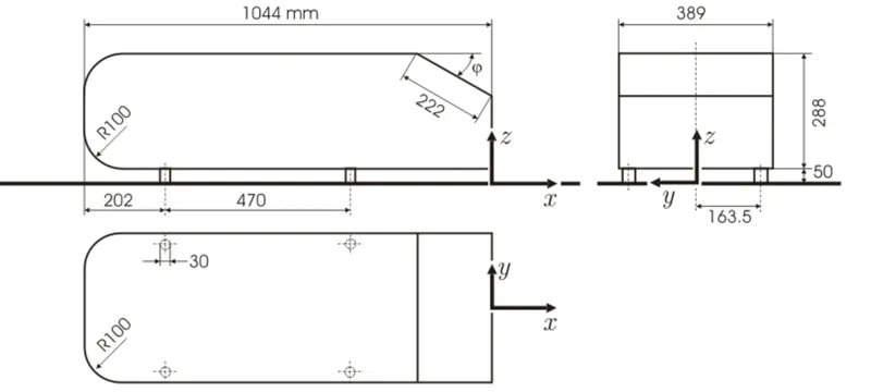
• Measurements superimposed on different three-dimensional viewing planes of the Ahmed Body model (all linear and angular dimensions are in mm and degrees)

Effect of Aspect Ratio: Venning et al [7] demonstrated that the rear slant's aspect ratio had a significant effect on the wake. The wider bodies stopped reattaching at 25° slant angles, indicating that the critical angle decreases as the aspect ratio increases. They also provide vortex core locations derived from experimental data for validation [8].

Description of the test case: The Ahmed body (Fig. 1) was first defined and its properties were described in Ahmed's experimental work [1]. As a test case, two configurations with slant angles of 25° and 35° are considered. Becker, Lienhart, and Stoots [2,3] conducted detailed LDA measurements in the LSTM low-speed wind tunnel for this configuration, with a cross-section of 1.87x1.4 m2 (width x height) and a bulk velocity of 40 m/s. The wind tunnel's test section was 3/4 open (only the ground plate was present). The body is 50 mm away from the plate representing the ground. Ahmed's experiment [1] used a flow velocity of 60 m/s and a Reynolds number of 4.29 million based on model length.

• Front View:

• Side view:

CASE SETUP:

GEOMETRY:

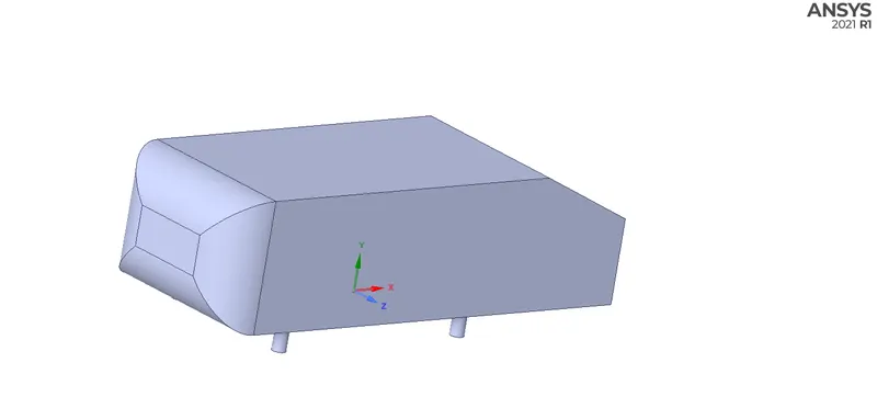
• Spaceclaim was used to create the geometry.
• It is saved as an STL file, which was then opened in Converge.
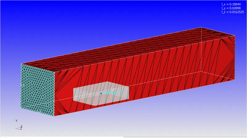
• Then, in the converge, a wind tunnel is created by creating Vertices and then patching them.
• The calculations were performed according to the scaling to determine the dimensions of the wind tunnel.

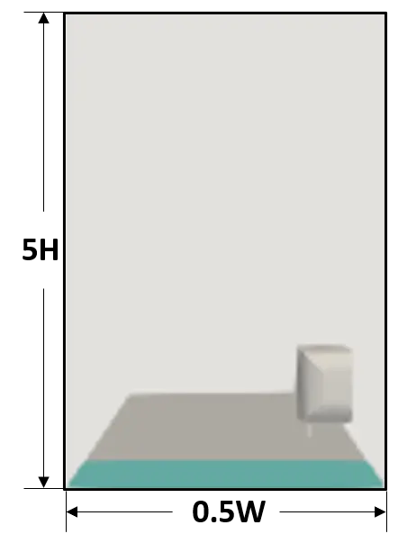
• As a result, a total distance of 2.3 metres is added from the geometry's front face to the inlet.
• The distance between the geometry's rear side and the outlet is set to 5 times the geometry's length, which is 5 metres.
• The typical values used by industries for this are between 5 and 10 times to effectively capture the physics by avoiding the interference of Outlet wall conditions. Because my current resources are limited, I will stick with the simplest solution (5 times)
• The Height is set to twice the geometry's length.
• The width has been set to 0.5 metres.
• At 400 mm in front of the Ahmed body, the boundary Layer Thickness is 30 mm.

• Application type: Time-based,
• Materials: air,
• Click on gas simulation as the air is gaseous state and click on species to calculate how the mass fraction of N2 and O2 are changing along the flow.
• A transient simulation is set,
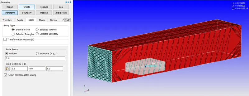
• Using the Transform option in converge, the scale is set to 0.1.

• Simulation time parameters:
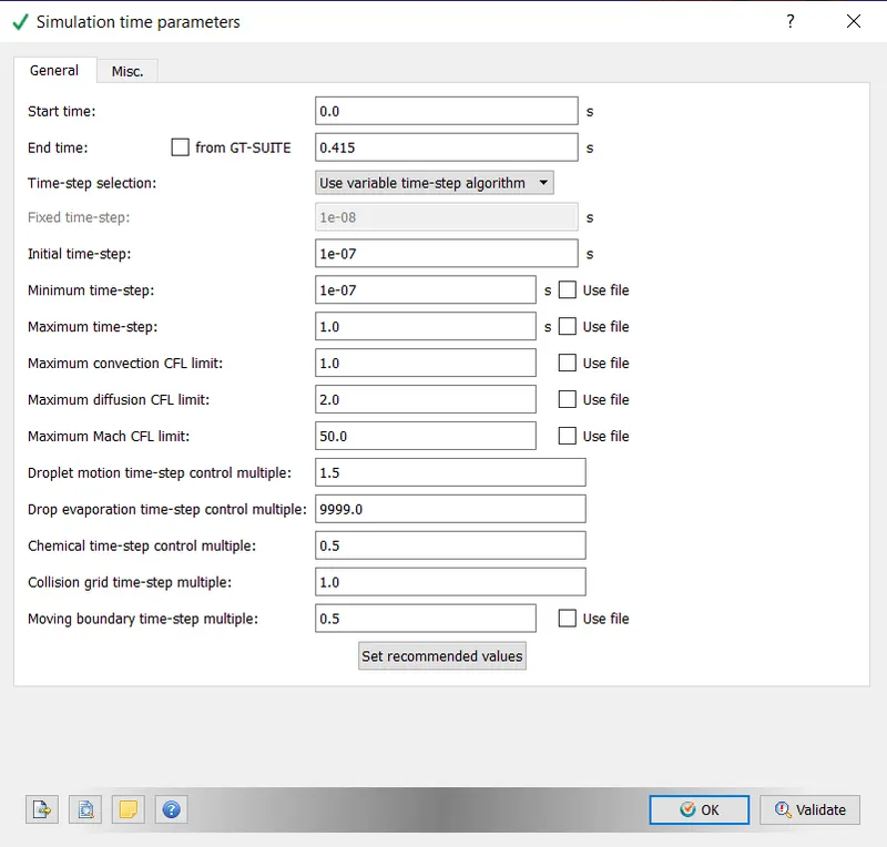
• The maximum convection cfl value should never be greater than or equal to 1. So that the solution would converge; otherwise, the solution would be blown up. I used the following procedure to calculate the end time.
• To calculate the time, we need velocity flow and elbow length. The wind tunnel here is 8.3 metres long. I chose a fluid with an inlet velocity of 40m/s. As a result, the time it takes the fluid to exit the wind tunnel is 0.2075 s. We need to set the simulation end time to two to five times the time it takes the fluid to exit the tunnel, so we can see the wake region and how the primitive variables got there.

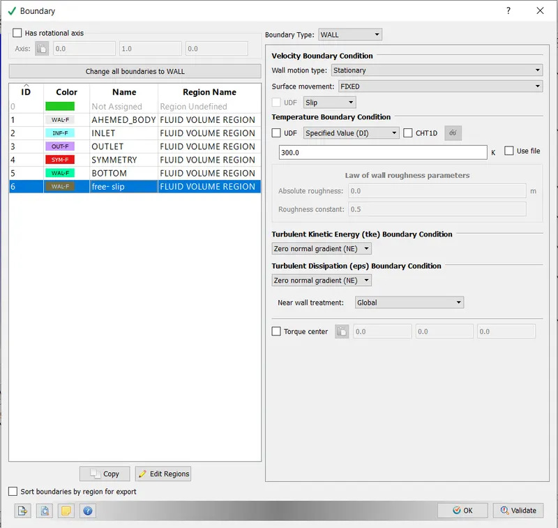
• The boundaries, such as the inlet, outlet, top and sidewalls, Free-slip wall, the law of the wall region, and the Ahmed body, are then appropriately highlighted.
• Regions and initialization: I've labelled the entire box region as a fluid volumetric region.

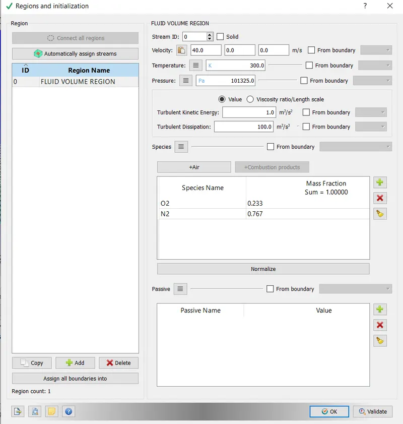
• The inlet velocity I've chosen is 40m/s.

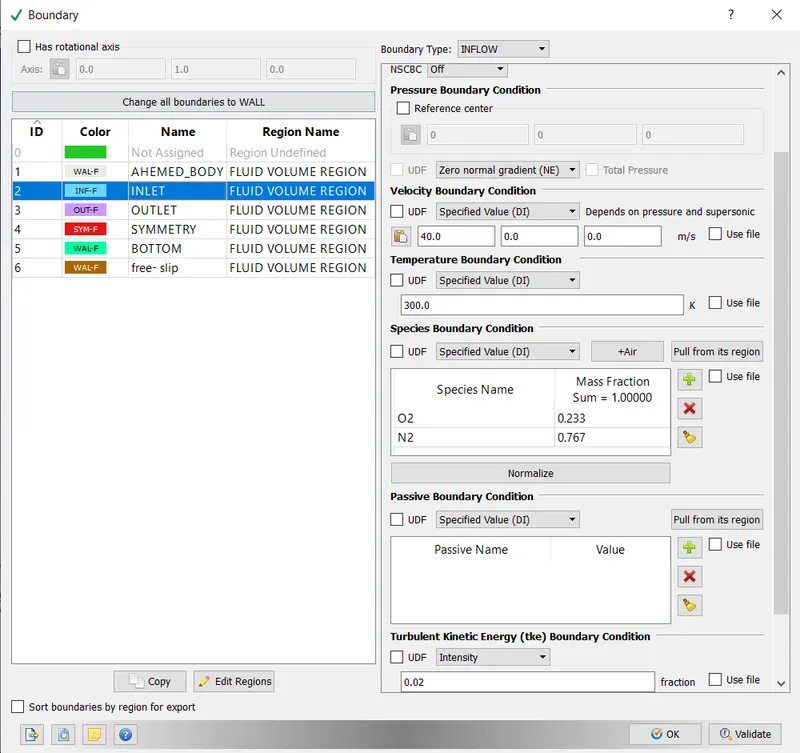
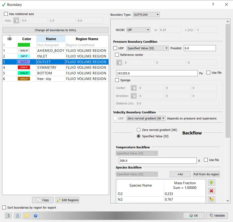
• Outlet- the atmospheric outlet pressure that I have taken is 101325 pascals.

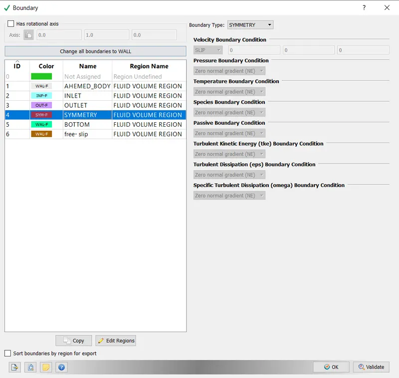
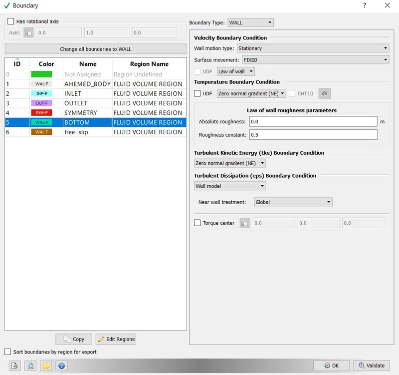
• Symmetry- I applied this boundary condition to all of the wing tunnel walls except the bottom of the wind tunnel.

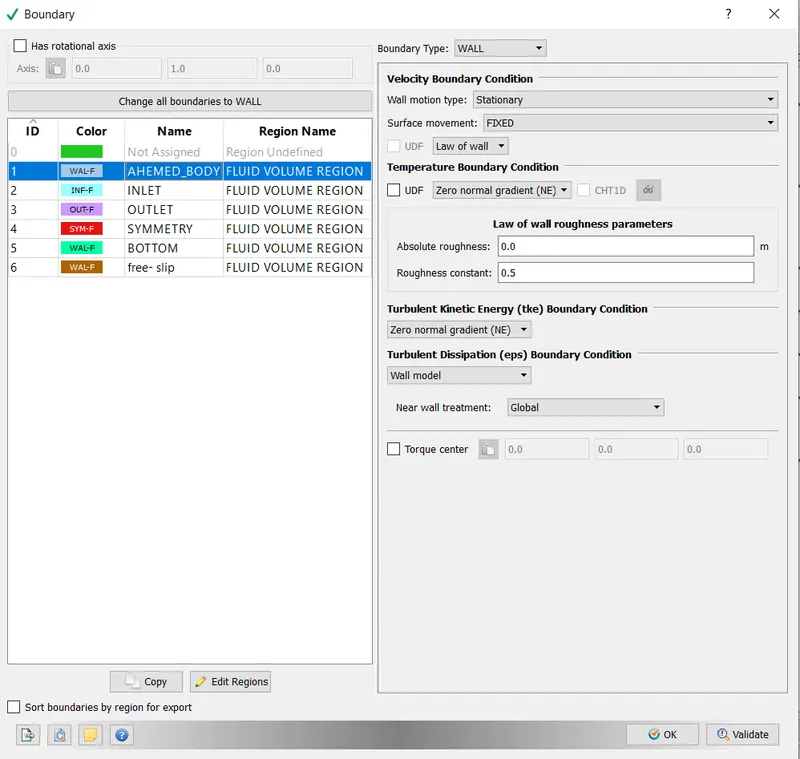
• Ahmed body:

• Bottom:

• Free Slip:

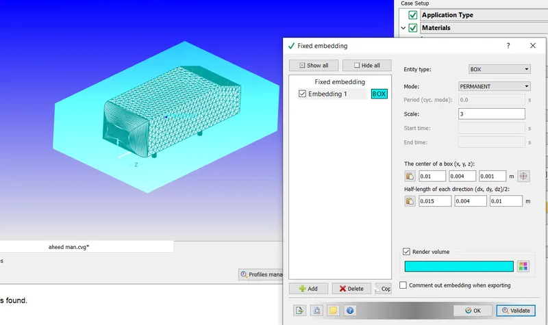
• Fixed embedding - I enabled fixed embedding in order to scale the cells at the geometry's walls. To capture turbulence in the turbulence boundary layer region, we must provide cells with small sizes at the boundary walls. The number of embedded layers represents the number of cell layers we will take. The scale represents what fraction of the base size is used for the first layer thickness. I calculated the scale using the following formula:
  first layer thickness = base size/2n, where n represents the scale.
• I reduced the scale that I obtained from the above formula because increasing the scale results in more refinement in the box, which increases the cell count. I only have limited access to the simulation's cell count. As a result, I've reduced the scale so that my software can begin the simulation.

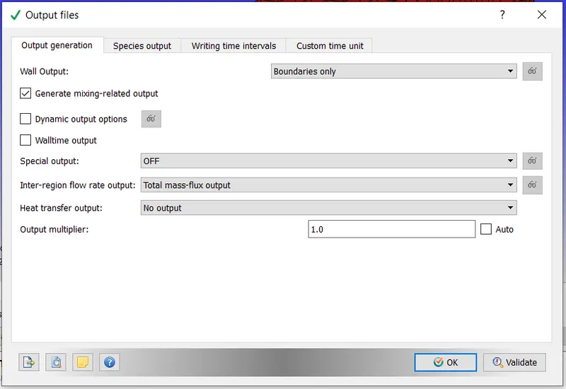
• Output/post-processing: Following variable selection, I enabled the y+ value in addition to the default variables.
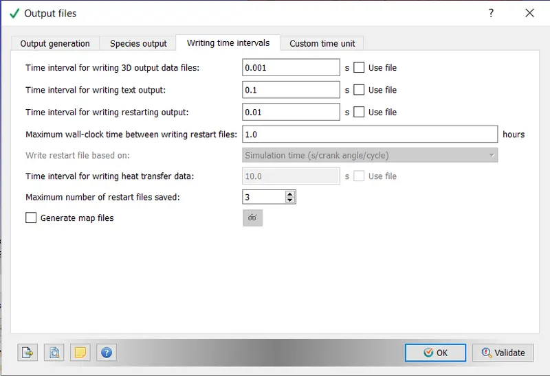
• output- The time interval between writing 3D output data files is 0.001 seconds. This means that the probe's output values are saved every 0.001 seconds. In the preview, we can see the values of primitive variables every 0.001 seconds. I've also enabled the boundary-only wall output to calculate the drag and lift focus acting on the body.

SOLUTION:

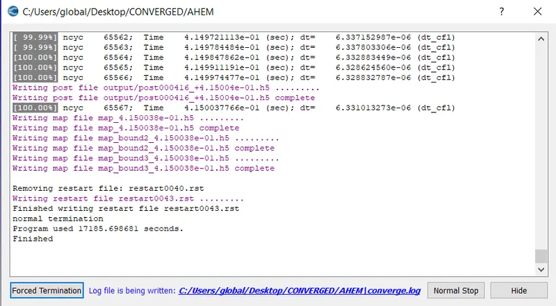
• Export all of the input files to a folder. As a result, we can conclude that converge is used to generate the simulation's input files.

RESULT:

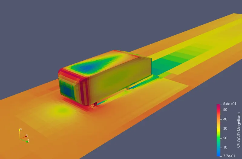
• VELOCITY CONTOUR:

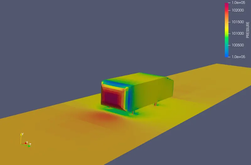
• PRESSURE CONTOUR:

• VELOCITY ANIMATION CONTOUR:

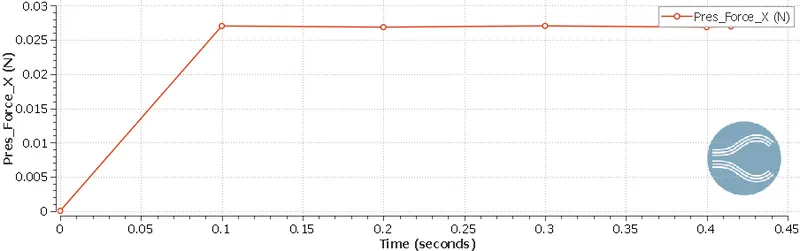
• Pressure Along X direction:

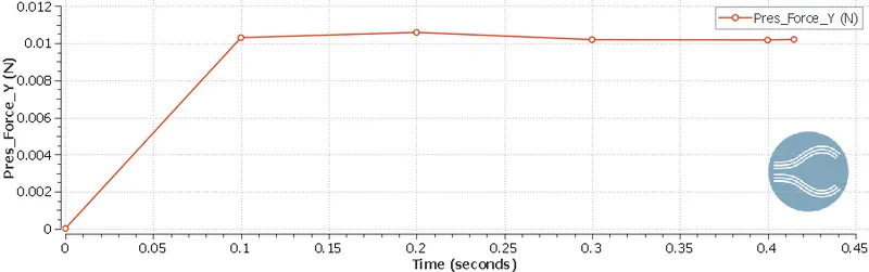
• Pressure Along Y direction:

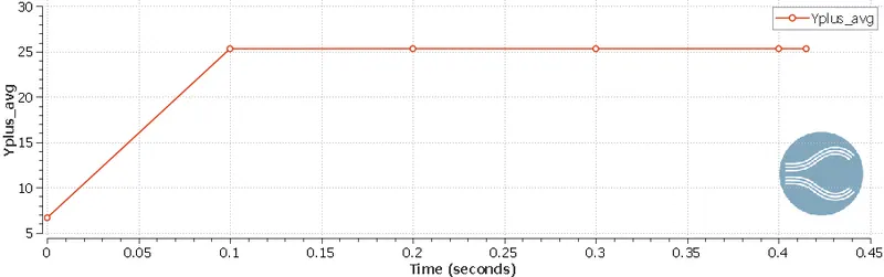
• Y- PLUS:

OBSERVATION:

• Because the y-plus average values are higher, the solutions are less accurate.
• To achieve high accuracy, the values must be smaller in order to capture the viscous sublayer.
• The wake regions at the rear are defined by the velocity contours.

CALCULATIONS USING ParaView:

• Drag and lift forces can be extracted from the paraview, and drag and lift coefficients can be calculated using the paraview calculator.
• To extract these forces, an Ahmed body block is extracted first, and then the surface is extracted after generating surface normals.
• The calculator is turned on, and pressure and normals x are multiplied in scalars to get drag force. Pressure is multiplied with normals z to get lift force.

• Now, in order to calculate the coefficient of drag, we need to know the frontal area that is opposing the flow. This area can be calculated using paraview.

Where,

Fd = 29.221 N

Cd = 2*29.221/(1.225*0.00943584*40^2) = 2.76

For the coefficient of lift,

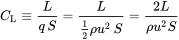
L = -105.26

S = 1.044*0.389 = 0.406

CL = (2*-105.26)/(1.225*0.406*40^2) = -0.316

VALIDATION:

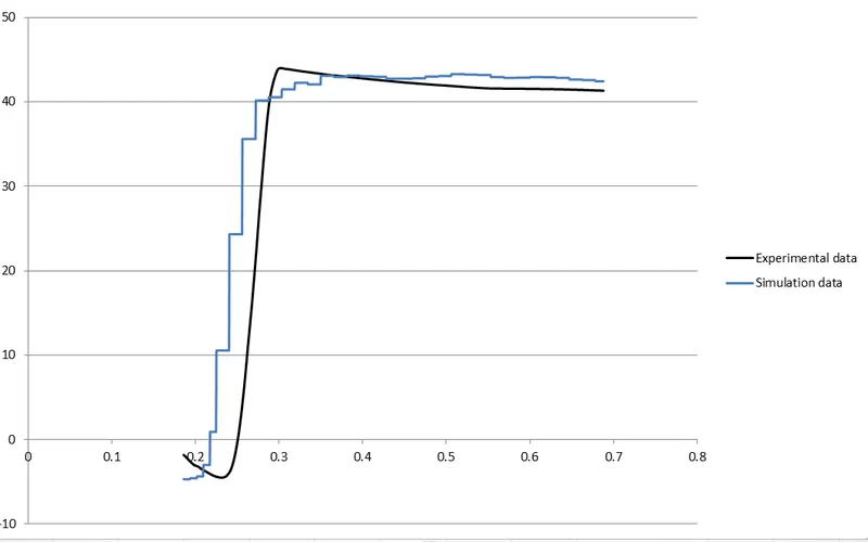
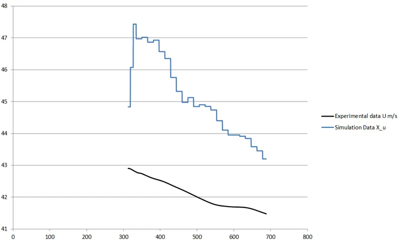
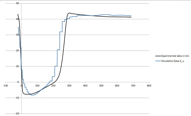
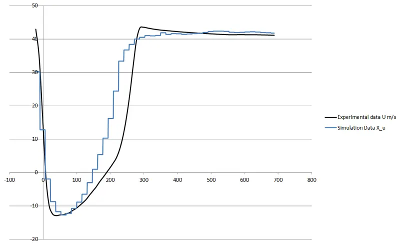
• To validate the extracted simulation data, experimental data is compared to it.
• The data are variations in velocity in the x-direction at various z-direction locations.
  Eight points were used, and these eight points are distributed across x.
• The experimental and simulated values are combined in the same Excel spreadsheet and plotted on the same graph.

Point-1 (X = -13 mm):

Point-2 (X = -263 mm):

Point-3 (X = 37 mm):

Point-4 (X = 87 mm):

Point-5 (X = -113 mm):

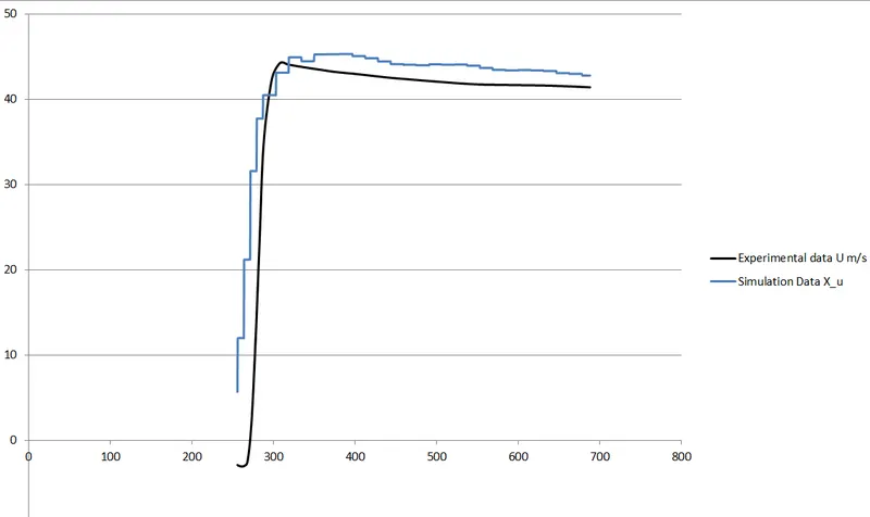
Point-6 (X = 63 mm):

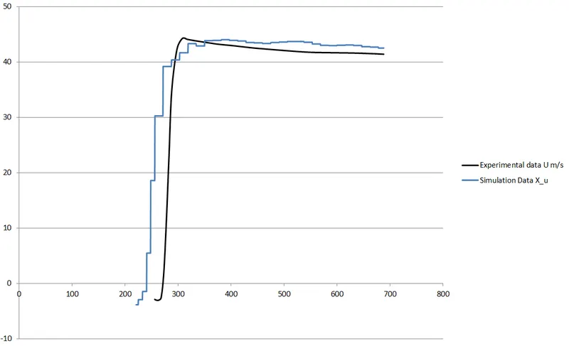
Point-7 (X = 187 mm):

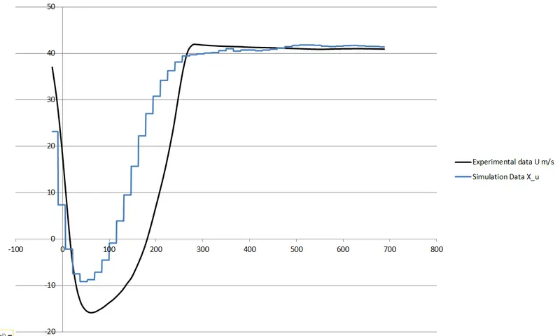
Point-8 (X = 137 mm):

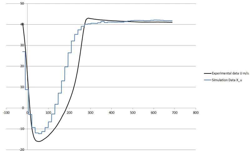
OBSERVATION:

• As previously stated, the simulation data and experimented data do not match at some points, owing primarily to the coarse mesh provided.
• Despite the fact that the results appear to be quite good, and the curves almost all follow the same slope,
• For validation, the difference between the experimental and simulated values must be less than 5%, but in my case, due to limited computational resources, the solutions are less accurate.

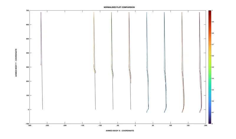
NORMALISATION:

• Done in order to visualise the change in simulation and experimental data.
• The data is calculated by combining the data from each x location, and the differences are then examined.
• It is first normalised before being multiplied by an amplification factor.
• It aids in determining the differences between the simulated and experimented data.
• The experimental data curve is black in colour.

CONCLUSION:

• The CAD model is created using SpaceClaim.
• Transient simulation of external flow over Ahmed's body.
• Post-processing and extraction Values for drag and lift force.
• Velocity contours extracted.
• Validated with experimental data by visualising velocity variation in the x direction at various z locations
• We can see from the pressure contour that there is an increase in pressure at the front face of the body due to a sudden drop in air velocity and a decrease in pressure at the back face of the body.
• The wake region is formed at the back base, and flow reversal also occurs at the rear portion of Ahmed's body.
• We can conclude from validation that using the coarse mesh will result in incorrect results.
• We also noticed that a negative lift force is generated here, which should be required for a moving body travelling on roads. There will be more traction if the negative lift force is increased so that the wheels of vehicles are always attached to the road.