Week - 10 Hyperelastic Material Models

Week - 10 Hyperelastic Material Models

Aim: Calculation of the Mooney Rivlin and Ogden material contstants and comparison of stress strain data is done using dogbone specimen.

Procedure:

Given data

Eng Strain	Eng Stress
0	0
0.025	0.0446
0.05	0.0867
0.075	0.127
0.1	0.164
0.125	0.2
0.15	0.234
0.175	0.267
0.2	0.298
0.225	0.328
0.25	0.356
0.275	0.383
0.3	0.409
0.325	0.434
0.35	0.458
0.375	0.481
0.4	0.503
0.425	0.524
0.45	0.545
0.475	0.565
0.5	0.584
0.525	0.603
0.55	0.62
0.575	0.638
0.6	0.655
0.625	0.671
0.65	0.687
0.675	0.702
0.7	0.717
0.725	0.732
0.75	0.746
0.775	0.76
0.8	0.773
0.825	0.786
0.85	0.799
0.875	0.811
0.9	0.823
0.925	0.835
0.95	0.847
0.975	0.858
1	0.869

This data is in Engineering Stress and Strain Data

LS DYNA:

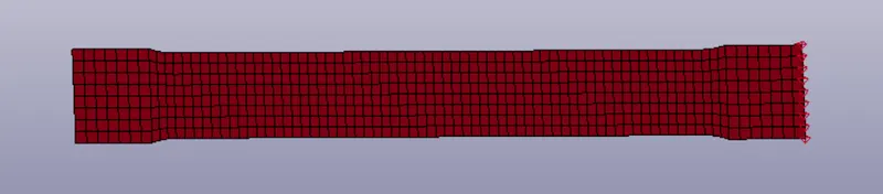
This above Eng stress ans strain data is using in simulating the given Dogbone specimen.

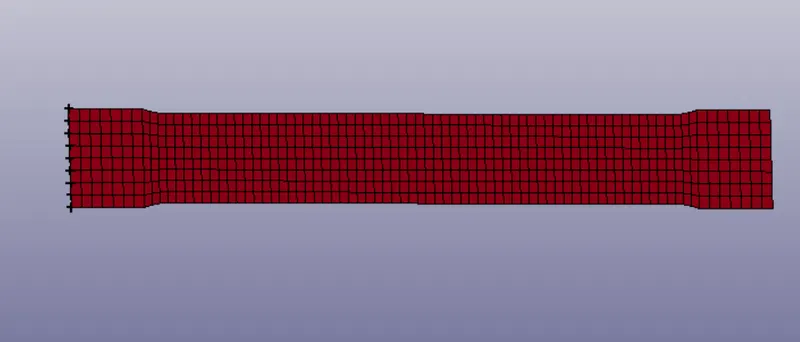
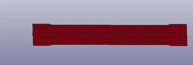
This specimen is opened in LS PrePost

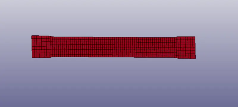
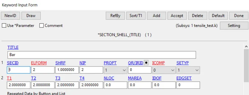
Necessary cards are generated for simulation

SECTION

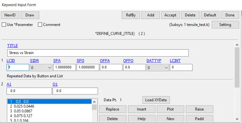
Material CURVE

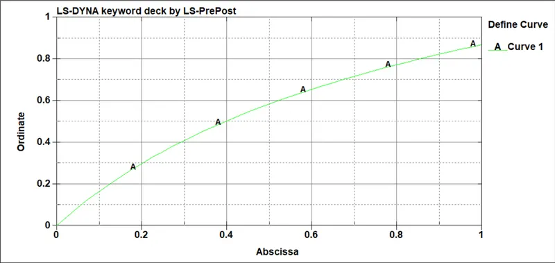
This Eng stress vs eng strain saved in csv format is loaded with LoadXY data

Plotting it we get,

MAT 77 H

The Mooney Rivlin material card has three variation for N =1, 2, 3 and so all three are used with different cases

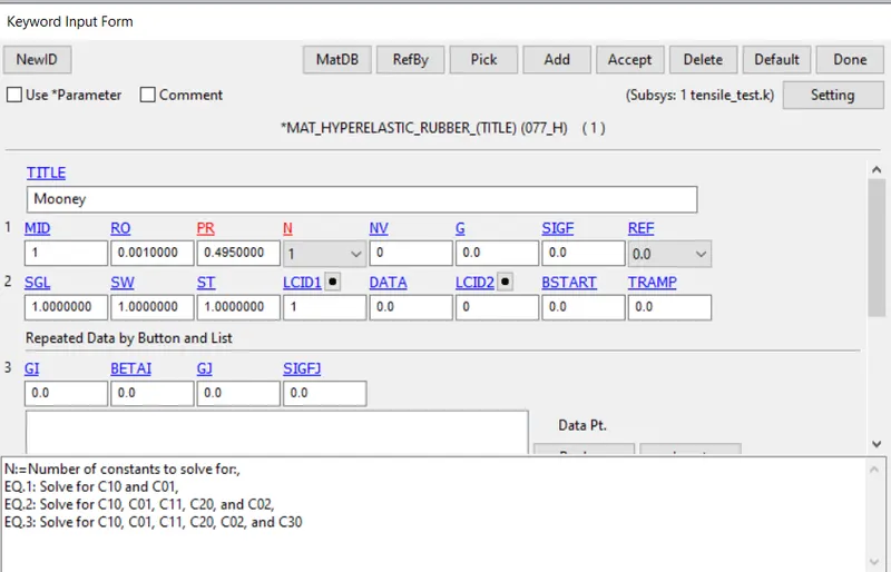
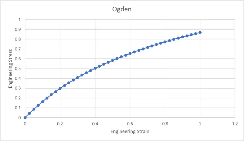
Similarly for Ogden material just N = 1 is taken

MAT 77O

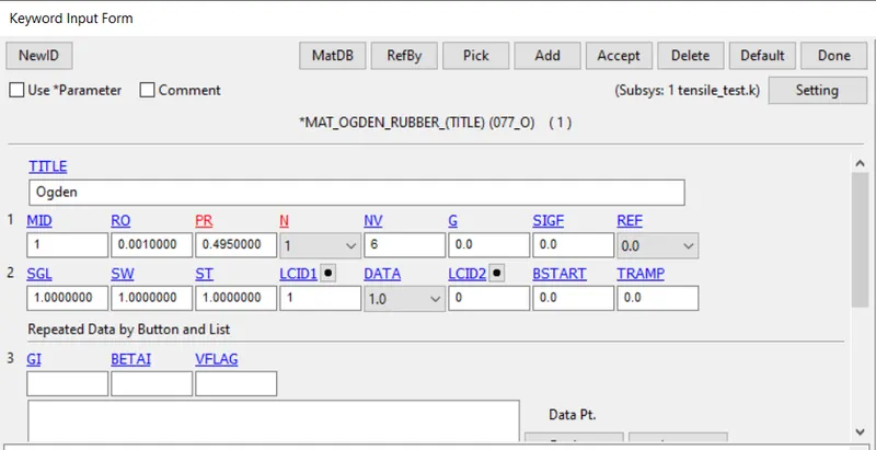
SGL, SW, ST are given 1 so that the curve in LCID1 has Engineering Stress vs strain data

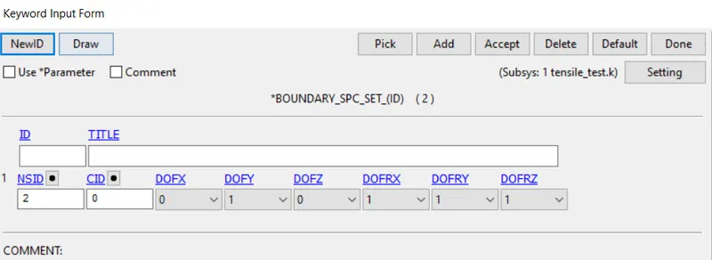
Boundary Conditions

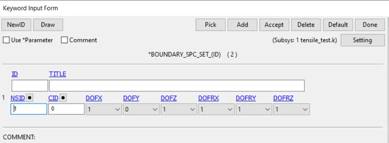
Fixing the nodes

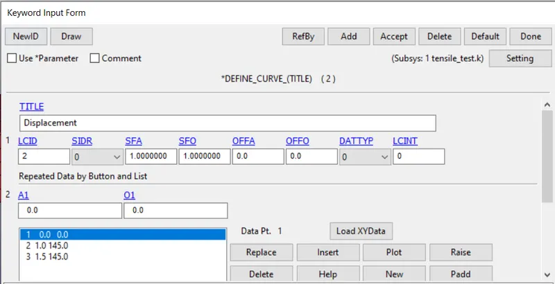
Displacement curve:

Giving displacement for 100 % strain and given specimen is of 145 mm

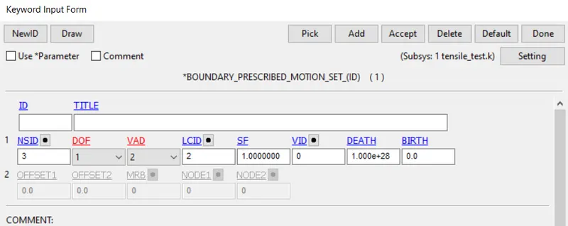
For displacement of nodes

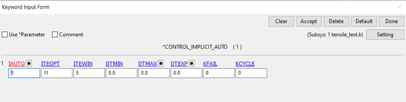
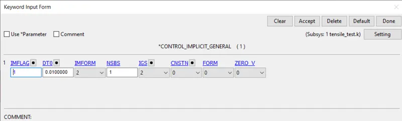
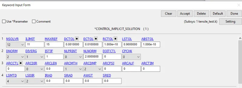
Since this quasistatic process IMPLICIT is activated

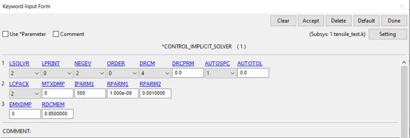
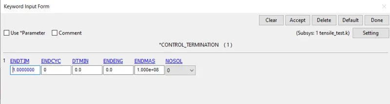
Termination time is given 1 ms

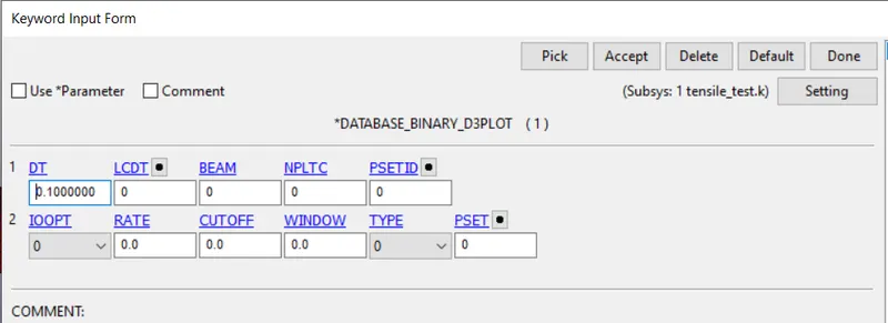
Output data:

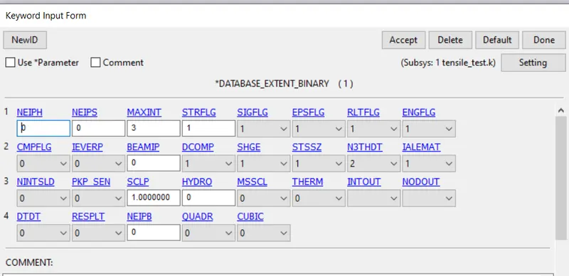
For strain data EXTENT_BINARY is activated with strflg = 1

In ASCII

ELOUT and GLSTAT is activated.

Then these 4 cases is run to get d3hsp file

Results:

From d3hsp files

For Monney Rivlin N = 1

For Monney Rivlin N = 2

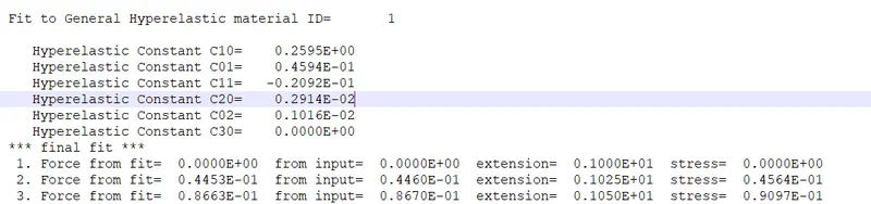
For Monney Rivlin N = 3

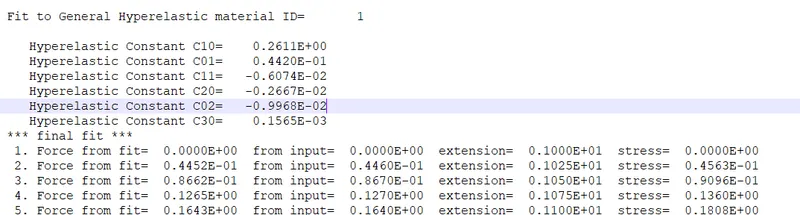
Here form above d3hsp files, extension is strech data and converting it to strain by

Extension = Strectch

Stretch = 1 + Engineering Strain

So conerting the True stress values to Engineering Stress, so we can plot Eng Stress vs Eng Strain data

Eng Stress = True Stress/(1+Eng Strain)

		Mooney Rivlin
Eng Strain	Eng Stress	N = 1		N = 2		N = 3		Ogden
0	0	0	0	0	0	0	0	0	0
0.025	0.0446	0.025	0.046927	0.025	0.044527	0.025	0.044517	0.025	0.044563
0.05	0.0867	0.05	0.090695	0.05	0.086638	0.05	0.086629	0.05	0.086679
0.075	0.127	0.075	0.131628	0.075	0.126512	0.075	0.126512	0.075	0.12655
0.1	0.164	0.1	0.17	0.1	0.164364	0.1	0.164364	0.1	0.164358
0.125	0.2	0.125	0.206133	0.125	0.200267	0.125	0.200267	0.125	0.200263
0.15	0.234	0.15	0.240261	0.15	0.234435	0.15	0.234435	0.15	0.234413
0.175	0.267	0.175	0.272426	0.175	0.266894	0.175	0.266979	0.175	0.266938
0.2	0.298	0.2	0.303	0.2	0.298	0.2	0.298	0.2	0.297959
0.225	0.328	0.225	0.331918	0.225	0.327592	0.225	0.327592	0.225	0.327582
0.25	0.356	0.25	0.35952	0.25	0.35592	0.25	0.35592	0.25	0.355907
0.275	0.383	0.275	0.385882	0.275	0.383059	0.275	0.383059	0.275	0.383022
0.3	0.409	0.3	0.411077	0.3	0.409	0.3	0.409	0.3	0.409009
0.325	0.434	0.325	0.43517	0.325	0.433962	0.325	0.433962	0.325	0.433943
0.35	0.458	0.35	0.458296	0.35	0.457926	0.35	0.457926	0.35	0.457891
0.375	0.481	0.375	0.480582	0.375	0.480945	0.375	0.480945	0.375	0.480917
0.4	0.503	0.4	0.502	0.4	0.503071	0.4	0.503071	0.4	0.503077
0.425	0.524	0.425	0.522667	0.425	0.524421	0.425	0.524421	0.425	0.524425
0.45	0.545	0.45	0.542621	0.45	0.545034	0.45	0.544966	0.45	0.545008
0.475	0.565	0.475	0.561966	0.475	0.564881	0.475	0.564881	0.475	0.564872
0.5	0.584	0.5	0.580667	0.5	0.584067	0.5	0.584067	0.5	0.584059
0.525	0.603	0.525	0.598885	0.525	0.602623	0.525	0.602623	0.525	0.602606
0.55	0.62	0.55	0.616516	0.55	0.620516	0.55	0.620516	0.55	0.620549
0.575	0.638	0.575	0.633714	0.575	0.638095	0.575	0.638095	0.575	0.637922
0.6	0.655	0.6	0.650625	0.6	0.655	0.6	0.655	0.6	0.654755
0.625	0.671	0.625	0.667077	0.625	0.670769	0.625	0.671385	0.625	0.671076
0.65	0.687	0.65	0.682424	0.65	0.686667	0.65	0.686667	0.65	0.686912
0.675	0.702	0.675	0.698507	0.675	0.70209	0.675	0.70209	0.675	0.702288
0.7	0.717	0.7	0.713529	0.7	0.717059	0.7	0.717059	0.7	0.717226
0.725	0.732	0.725	0.728696	0.725	0.731594	0.725	0.731594	0.725	0.731749
0.75	0.746	0.75	0.742857	0.75	0.745714	0.75	0.745714	0.75	0.745877
0.775	0.76	0.775	0.757746	0.775	0.759437	0.775	0.759437	0.775	0.759628
0.8	0.773	0.8	0.771667	0.8	0.772778	0.8	0.772778	0.8	0.77302
0.825	0.786	0.825	0.785205	0.825	0.786301	0.825	0.786301	0.825	0.78607
0.85	0.799	0.85	0.798919	0.85	0.798919	0.85	0.798919	0.85	0.798794
0.875	0.811	0.875	0.812267	0.875	0.8112	0.875	0.8112	0.875	0.811205
0.9	0.823	0.9	0.825789	0.9	0.823158	0.9	0.823158	0.9	0.823319
0.925	0.835	0.925	0.838442	0.925	0.835325	0.925	0.835325	0.925	0.835147
0.95	0.847	0.95	0.851282	0.95	0.846667	0.95	0.846667	0.95	0.846702
0.975	0.858	0.975	0.864304	0.975	0.858228	0.975	0.858228	0.975	0.857996
1	0.869	1	0.8765	1	0.869	1	0.869	1	0.86904

Comparison Plots for above Stress strain data:

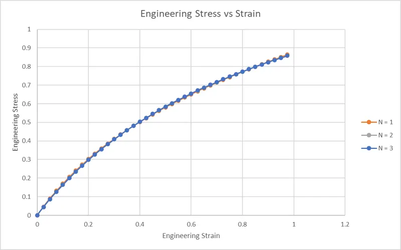
Ogden Graph

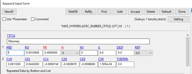
For validation og given results with the calculated constants, we input the constants from N =3 in

Material card of MAT 77 N = 0

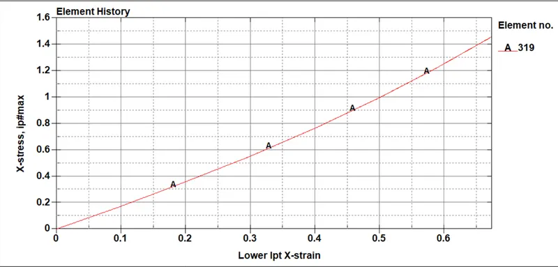
After the simulation is run using cross plot we get True Stress Strain data

converting it to eng stress and strain and comapring with the given data we get

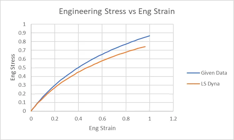
We can see that simulated Area of reduction is more compared to given data.

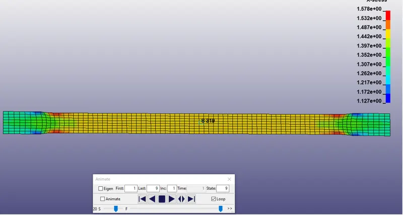
The contour of X stress

Conclusion:

The given Stress strain curve is converted to material data and is validated with given Dogbone specimen.

Intially the Dogbone specimen is opened in LS PrePost