Week - 10 Hyperelastic Material Models

Hyperelastic material modelling from raw data and determination of different coefficients

1. Introduction

A general material is elastic up to 0.2% strain but in the case of hyperelastic materials, they can get up to 500% strain and still come back to their original shape.

Modelling of a hyperelastic material becomes difficult in comparison to the elastic materials as the model needs to take care of non-linear material behaviour as well as the large shape change.

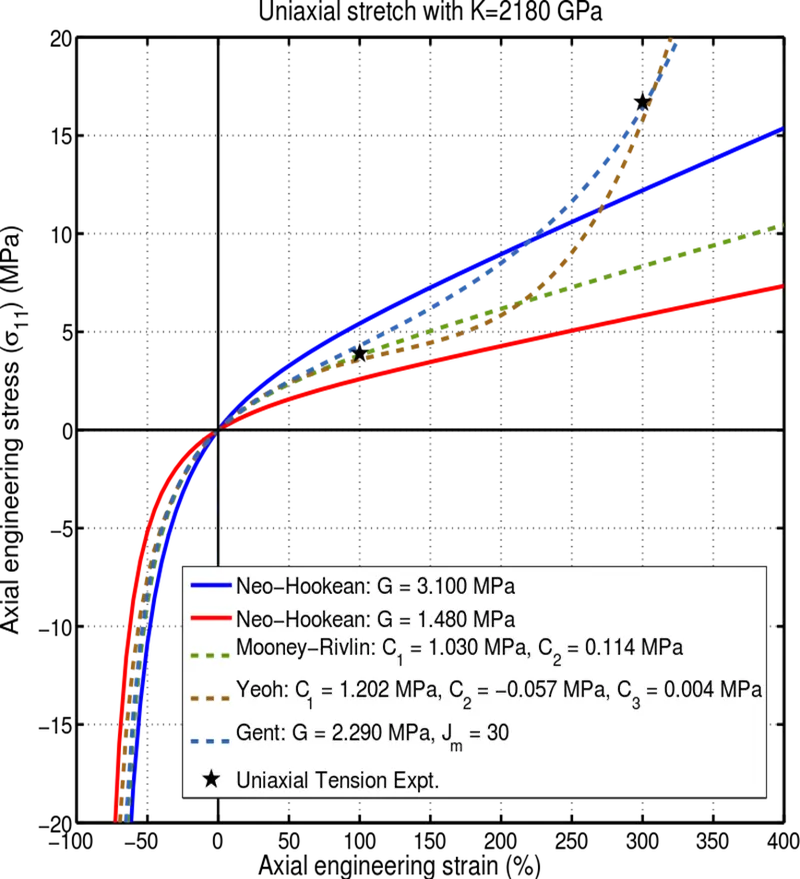
Fig 1.0: The typical stress-strain curve for hyperelastic materials.

The linear part of the curve is minuscule and the elastic modulus is in the 0.1 to 100 MPa. Another important point is, even the non-linear portion in the curve behaves in an elastic manner which makes it incompatible with the elastic-plastic model.

Since this material model needs to account for both, the non-linear material behaviour as well as large shape changes, this behaviour is described in the terms of strain energy as a function of stretch. The most common examples are rubber, foam and adhesives.

Stretch can be defined as `lambda=(Deltal+L)/L` and this translates to `epsilon= (lambda-1)` where `lambda, L, Delta l, epsilon` are stretch, initial length, change in length and engineering strain. When the stretch is 1 there is no deformation. At `lambda=2` we have 100% strain.

Further, strain energy can be defined as energy stored by the system while undergoing deformation. Mathematically, `U=1/2*v*sigma*epsilon` where U, v,`sigma, epsilon` are strain energy per unit volume, volume, engineering stress and engineering strain respectively.

Strain energy per unit volume is termed strain energy density. This strain energy density can be expressed as functions of principal stretch and deformation tensor.

There are different hyperelastic constitutive laws, some of them are:

• Neo-Hookean (1st order reduced polynomial)
• Mooney-Rivlin (1st order polynomial)
• Yeoh (3rd order polynomial) - generalised form is `W= Sigma_(i,j=0)^(n) C_(ij)*(I_1-3)^i*(I_2-3)^j + (Extra term for compressibility)` where W is strain energy density, C represents hyperelastic constants and I represents strain invariants.

In LS-Dyna basically, two material cards are used for modelling hyperelastic material; (1.) Mat_hyperelastic rubber_077 and (2.) Mat_hyperelastic rubber_077-Ogden.

In this exercise, a Mat_077_H card was used to model a hyperelastic material from engineering stress-strain data. The fitted curve obtained by the solver was compared against original data and the original data was also checked with the tensile test data of a dogbone specimen. The complete procedure is explained in the following sections:

2. The hyperelastic material card in the LS-Dyna

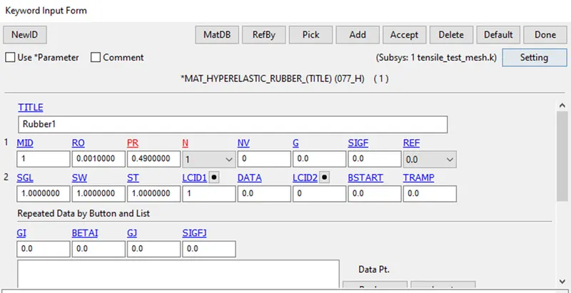
Fig 2.1: The hyperelastic material card in the LS-Dyna

In the above card, the model used for material behaviour can be chosen by selecting 'N' values. N=1 gives Mooney Rivlin rubber model and uses constants C01 and C10. The complete list of coefficients is calculated against N values when we enter the Engineering stress-strain data as a curve under LCID.

The Engineering stress-strain data provided as part of this exercise is shown in the attached figure below.

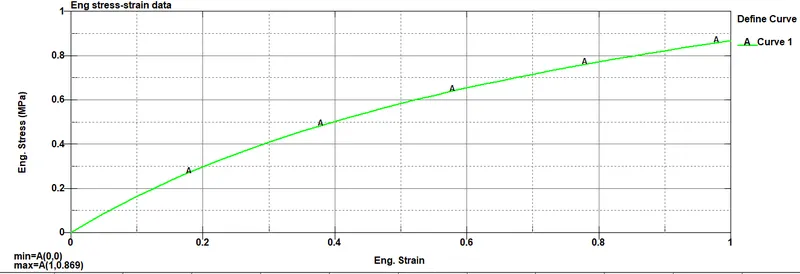
Fig 2.2: The Engineering stress-strain data provided for the rubber material

• The number of hyperelastic constants to solve for from LCID1:
• EQ.1: Solve for C10 and C01
• EQ.2: Solve for C10, C01, C11, C20, and C02
• EQ.3: Solve for C10, C01, C11, C20, C02, and C30

After that, the values of the calculated constants can be looked for in the d3hsp file available in the output files written by the solver. Then these values can be directly used with corresponding N values without the need of entering the entire engineering stress-strain values.

In this exercise, all the approaches of using N values 1,2,3 were adopted and the outcome of each test was compared with the original test data as explained in the following sections:

3. Evaluation of constants

A tensile test of the dogbone specimen was set up as shown in the attached figure for running a few iterations of the solution.

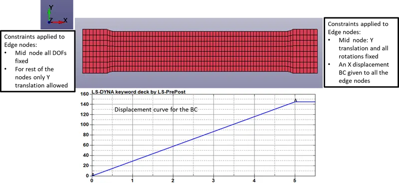
Fig 3.1: The model used for tensile test simulation of the dogbone specimen

The provided data shows an extreme strain value as 100% strain, so in the boundary conditions, a total displacement of 145 mm, which is equal to specimen length was used as a boundary condition.

The simulations were run with N values as 1, 2 and 3 respectively with the material card as shown in figure 2.1. After the solution is initialised, a d3hsp file is written in the parent folder of the model and this file can be referred to for finding the fitted curve (true stress vs stretch) that was used by the solver as well as the different constants.

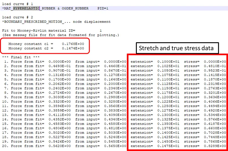
Fig 3.2: Snippet from the d3hsp file for N=1 material model.

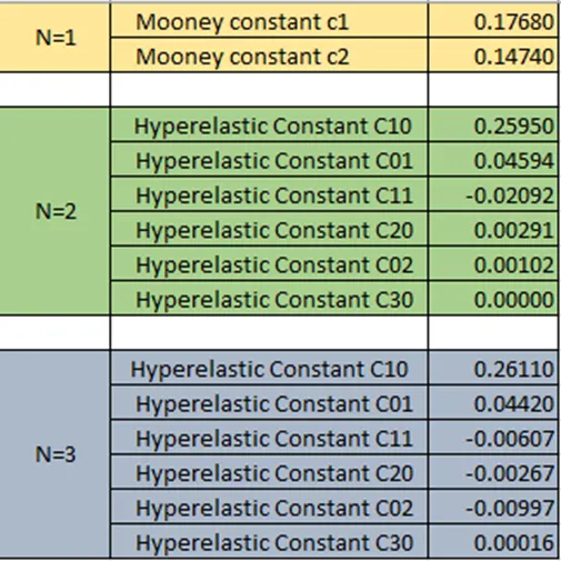
Table 3.1: Different hyperelastic constants obtained

After that, the true stress vs stretch data was converted to engineering stress-strain data using the following general formulae:

• `epsilon_t=ln(1+epsilon)` where `epsilon_t and epsilon` are true strain and engineering strain respectively.
• `sigma_t=sigma*(1+epsilon)` where `sigma and sigma_t` are the true stress and engineering stress respectively.
• `epsilon = lambda-1` where `lambda` is the stretch ratio.

Then a comparison with the original data was made by plotting them on a scatter chart as shown in the attached figure.

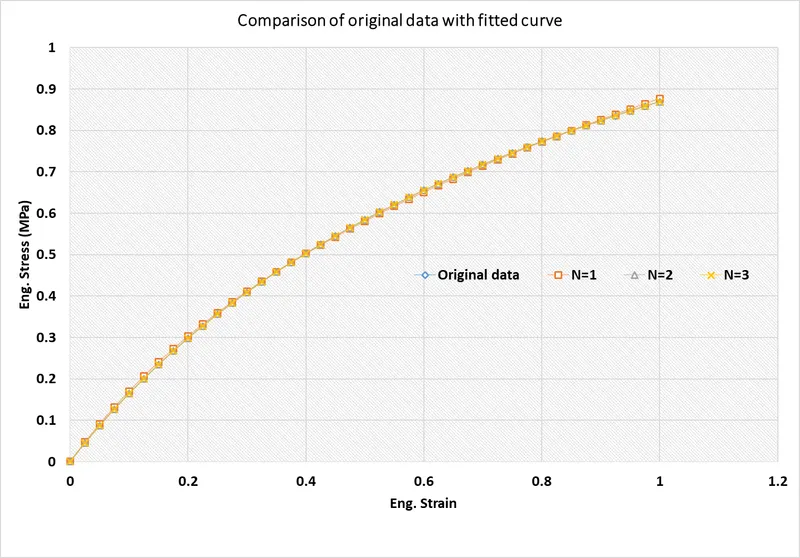
Fig 3.3: The comparison of fitted curves used by the solver for different N values

As clear from the plot the fitted curves for all the N values were almost the same and were fitting closely to the provided data. The next phase of the exercise was to evaluate these values with simulation results for the tensile tests on the dogbone specimen.

4. Test result for the tensile test

In this part of the exercise, the test results were obtained by running the simulations using an implicit scheme and the stress-strain data were compared with the original data.

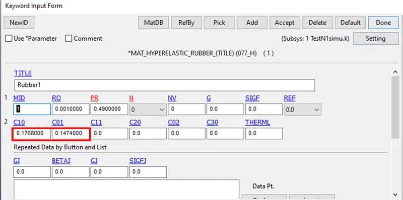
Fig 4.1: The material card settings used to model the Mooney-Rivlin model by entering C10 and C01 values with N=0

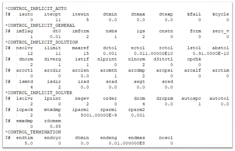
Fig 4.2: The implicit solver settings used for the model

Similarly, all other cases pertaining to N=2 and 3 were modelled and stress-strain data were extracted for an element.

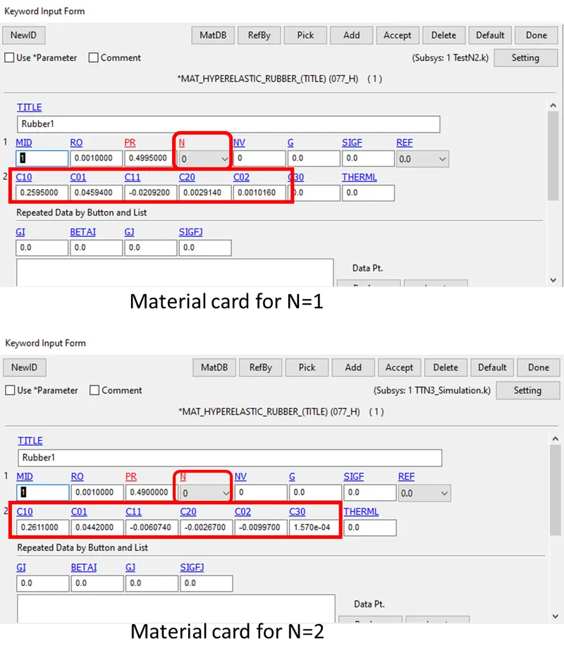
Fig 4.3: The material cards used for N=2 and 3

The comparison is plotted in the below-given plot.

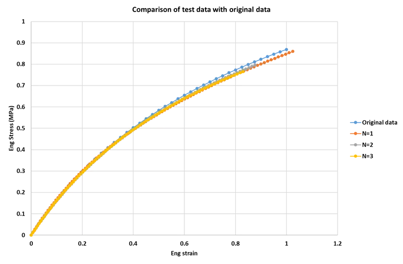
Fig 4.4: the comparison of test data with the original data for the rubber material

As clear from the plot, a slight deviation from the original data can be observed. This can be attributed to the fact that the stress-strain data entered in the material card of hyperelastic rubber should contain values for compression as well. In our case, there was no compression data in the engineering stress-strain data.

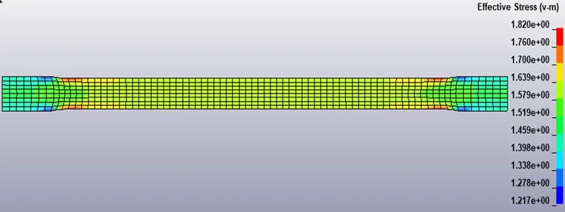
Fig 4.5: the effective stress contour

This contour plot can be used just as a means to verify that there are no steep stress gradients or concentrations in the geometry.

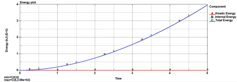
Fig 4.6: the energy plots for the simulation

AS evident from the plot, the internal energy of the system increases due to strain work being done on the system which validates the results up to a good extent.

5. Conclusion

• Material modelling involves cleanup of raw data, obtaining a fitted curve and then using a proper material card according to material behaviour. Then comes the validation of the model using coupon level followed by sub-assembly level testing of the material model and verification against test data.
• The fitted curve in the case of hyperelastic models is quite difficult to find manually unlike the elastic-plastic material curves. This is done by the LS-Dyna itself which uses an inbuilt algorithm to evaluate a fitted curve that can be seen from the d3hsp file.