Week - 10 Hyperelastic Material Models

AIM:

The objective of the report is to perform tensile test for hyperelastic materials by using Mooney Rivlin and Ogden material models and validate the results.

ABSTRACT:

HYPER ELASTIC MODELS -

In plastic elastic materials, the elastic behavior is seen till up to 0.2% of total deformation. Generally, in these materials, the elastic behavior is validated by using linear Hooke's law. 

In, Hyper elastic materials, the elastic behavior is seen till up to 500% deformation. So, it is not possible to validate the hyper elastic model with hooke's law as non linearity also exists in these models.

Constitutive laws for hyper elastic models - 

Many laws have been proposed to validate hyper-elasticity

Some famously used hyperelastic models are - 

1. Mooney-Rivlin - (1st order polynomial)
2. Neo-Hookean - (1st order polynomial)
3. Yeoh & Fleming - (3rd order polynomial)
4. Ogden 

These consecutive laws, strain energy density function is used to describe the model from which stress-strain relations are derived - 

1) For first three models, the energy density function are expressed in terms of variants

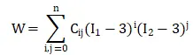, where W - Strain energy density function, I - invariants, Cij - Material constants,                                                                           n - order of polynomial

a) n = 1, indicates 1st order polynominal. Material constants - C10, C01 

b) n = 2, indicates 2nd order polynominal. Material constants - C10, C01, C11, C20, C02

c) n = 3, indicates 3rd order polynominal. Material constants - C10, C01, C11 ,C20 ,C02, C30  

2) For Ogden material model, the strain energy density function is expressed in terms of principal stretches.

, where  W - Strain energy density function, λ - Principal stretch,                                                                                                   (N, μp, αp) - Material constants  

1. N = 3, material behavior of rubbers can be described accurately
2. N =1, α1 =2 , Ogden material model is reduced to Neo-Hookean solid model
3. N =2, α1 =2, α2 =-2, Ogden material model reduced to Mooney-Rivlin material model

PROCEDURE:

In order to model the hyperelastic model in LS-DYNA, the material card has to be modeled by using experimental data.

STEP 1 - Extract the given eng-stress, eng-strain data into excel sheet 

Given, experimental data - units:MPa

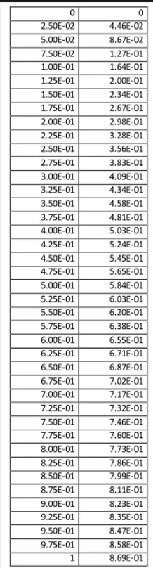
Convert the above data into kg-mm-ms and define the curve in LS-DYNA in .csv format

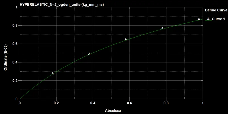
STEP 2 - Input the required keywords in LS-DYNA

(a) material card for MOONEY_RIVLIN_N1 -

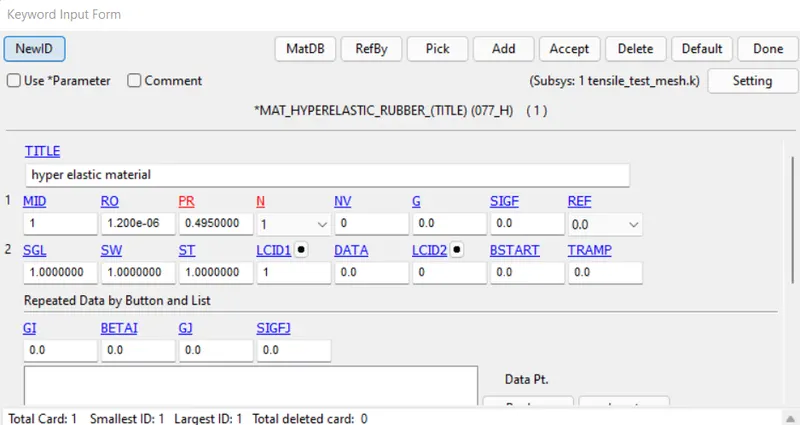
Similarly we can define for different constants - N = 2,3.

material card for OGDEN_N3

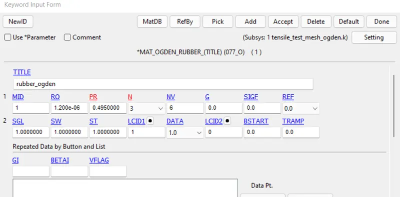
Similarly we can define for different constants - N = 1,2.

(b) BOUNDARY CONDITIONS - 

Fixing left end of the specimen in x-direction

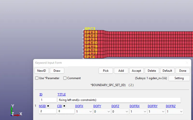
Fixing middle plane

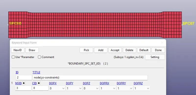
Prescribed motion to the right end of specimen

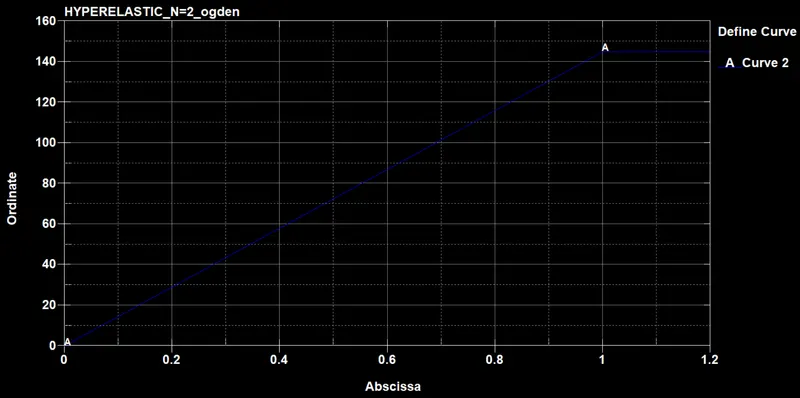
(c) IMPLICIT CONTROL CARDS - 

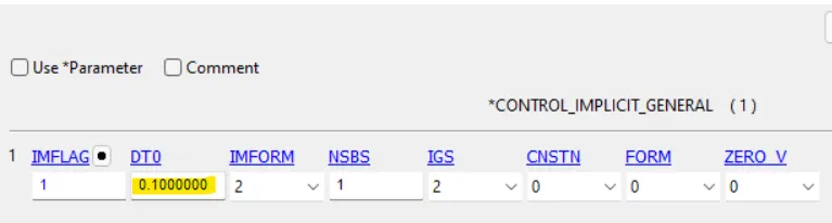
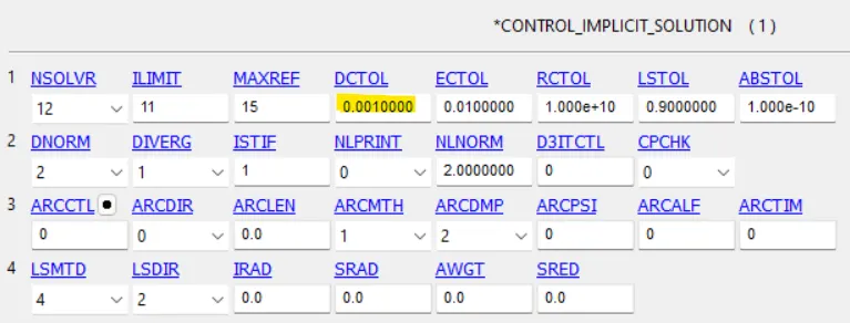
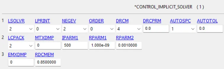
STEP 3 - POST PROCESSING

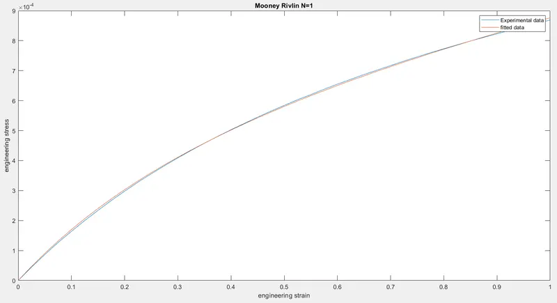
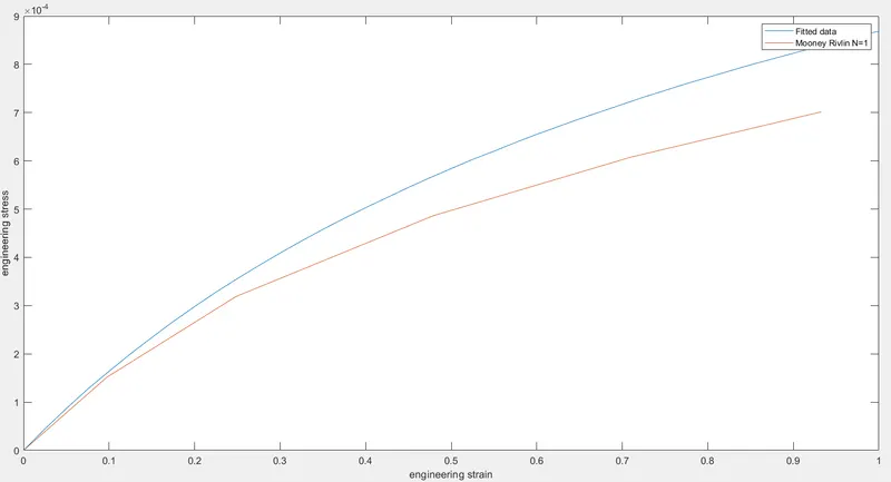
Hyper elastic model - n=1

Mooney constant c1 = 0.1768E-03
Mooney constant c2 = 0.1474E-03

The following graph shows the experimental data v/s fitted data obtained from d3hsp file.

The following graph shows the experimental data plot v/s simulated results 

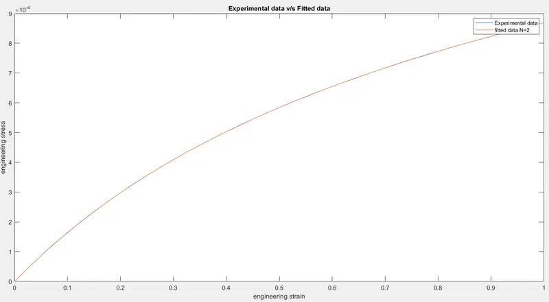
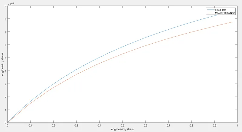
Hyper elastic model - n=2

Hyperelastic Constant C10= 0.2595E-03
Hyperelastic Constant C01= 0.4594E-04
Hyperelastic Constant C11= -0.2092E-04
Hyperelastic Constant C20= 0.2914E-05
Hyperelastic Constant C02= 0.1017E-05
Hyperelastic Constant C30= 0.0000E+00

The following graph shows the experimental data v/s fitted data obtained from d3hsp file.

The following graph shows the experimental data plot v/s simulated results 

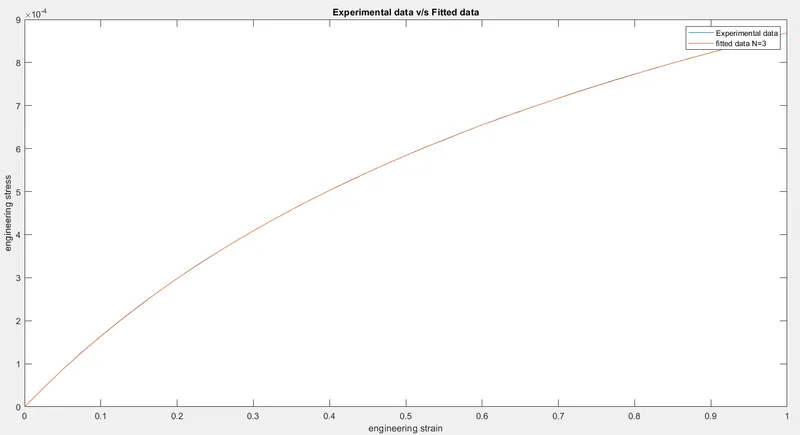
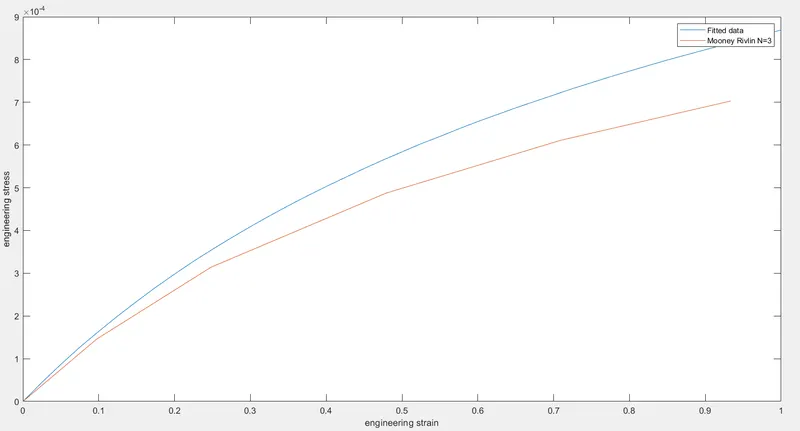
Hyper elastic model - n=3

Hyperelastic Constant C10= 0.2611E-03
Hyperelastic Constant C01= 0.4420E-04
Hyperelastic Constant C11= -0.6077E-05
Hyperelastic Constant C20= -0.2666E-05
Hyperelastic Constant C02= -0.9966E-05
Hyperelastic Constant C30= 0.1565E-06

The following graph shows the experimental data v/s fitted data obtained from d3hsp file.

The following graph shows the experimental data plot v/s simulated results 

Ogden material model - n=3

mu(1)=-3.1842708822766E-05 alpha(1)= 1.9262961084057E+00
mu(2)= 2.6137539678078E-04 alpha(2)= 1.5503244215991E+00
mu(3)= 6.8199166678390E-04 alpha(3)= 1.2887877438960E+00

The following graph shows the experimental data v/s fitted data obtained from d3hsp file.

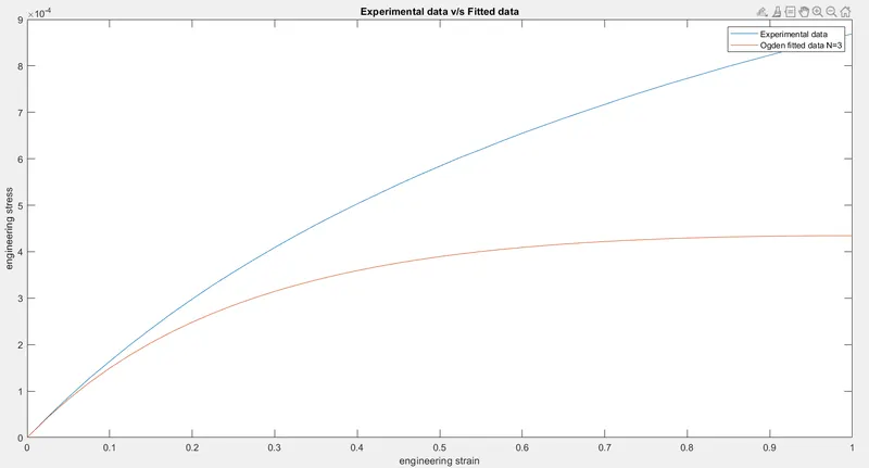
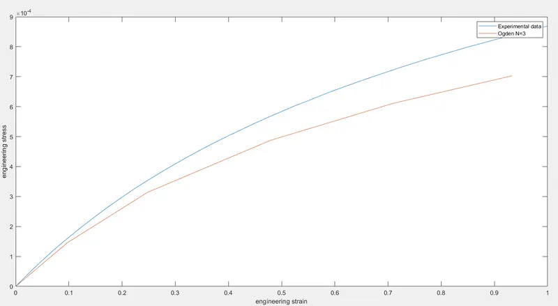
The following graph shows the experimental data plot v/s simulated results 

CONCLUSION:

Since, the analysis is done by using Implicit solver, the accuracy of the obtained results depends on the time step value.