Week 1- Mixing Tee

Aim: The aim of the study are the following

1. Analyze the mixing based on the inlet properties like velocity and temperature

2. How different turbulence physical models affect the results

3. Mesh convergence study

4. analyze the mixing T for understanding how the flow mixing works

Introduction and Theory:

T-joints are formed using two different pipe section combined at right angles. There are two inlet section from where two fluids will be mixed and pass through the outlet.

T joints are one of the most important joint in the piping network. The T joints are there to either combine the flow or divide the flow. The practical applications for mixing are nuclear powerplants, heating and ventilations section for buildings, liquid natural gas production and transportation etc...

Physical models that are being used in these simulations are

1.K-epsilon model

2. K-omega model

1. 𝑘−𝜖 model:

The K-epsilon model is based on the turbulent viscosity hypothesis. The model is complete and versatile.

This model is used to rank the performance of fluid system designs before experimental tests are taken.

Limitations on its accuracy arise from the turbulent viscosity hypothesis, 𝜀 equation, and wall functions when they are used.

2. 𝑘−𝜔 model

This model is developed by wilcox in 1993.In this model the expressions for 𝜈_𝑇(turbulent viscosity) and the 𝑘 equation are the same as those in the 𝑘−𝜖 model.

Now we will start the process of analyzing the given data to see no.of simulations

case 1: short Tee

case 2: Long Tee

Case 1: MR(Momentum Ratio) =2 Hot Inlet velocity =3m/s Based on the formula given Momentum ratio = velocity at cold inlet / velocity at hot inlet cold inlet velocity =6 m/s Model =𝑘−𝜖	Case 1: MR(Momentum Ratio) =4 Hot Inlet velocity =3m/s Based on the formula given Momentum ratio = velocity at cold inlet / velocity at hot inlet cold inlet velocity =12 m/s Model =𝑘−𝜖
Case 1: MR(Momentum Ratio) =2 Hot Inlet velocity =3m/s Based on the formula given Momentum ratio = velocity at cold inlet / velocity at hot inlet cold inlet velocity =6 m/s Model =𝑘−𝜔	Case 1: MR(Momentum Ratio) =4 Hot Inlet velocity =3m/s Based on the formula given Momentum ratio = velocity at cold inlet / velocity at hot inlet cold inlet velocity =12 m/s Model =𝑘−𝜔
Case 2: MR(Momentum Ratio) =2 Hot Inlet velocity =3m/s Based on the formula given Momentum ratio = velocity at cold inlet / velocity at hot inlet cold inlet velocity =6 m/s Model =𝑘−𝜖	Case 2: MR(Momentum Ratio) =4 Hot Inlet velocity =3m/s Based on the formula given Momentum ratio = velocity at cold inlet / velocity at hot inlet cold inlet velocity =12 m/s Model =𝑘−𝜖

Also in the short tee cases and long tee cases there are mesh independent studies.

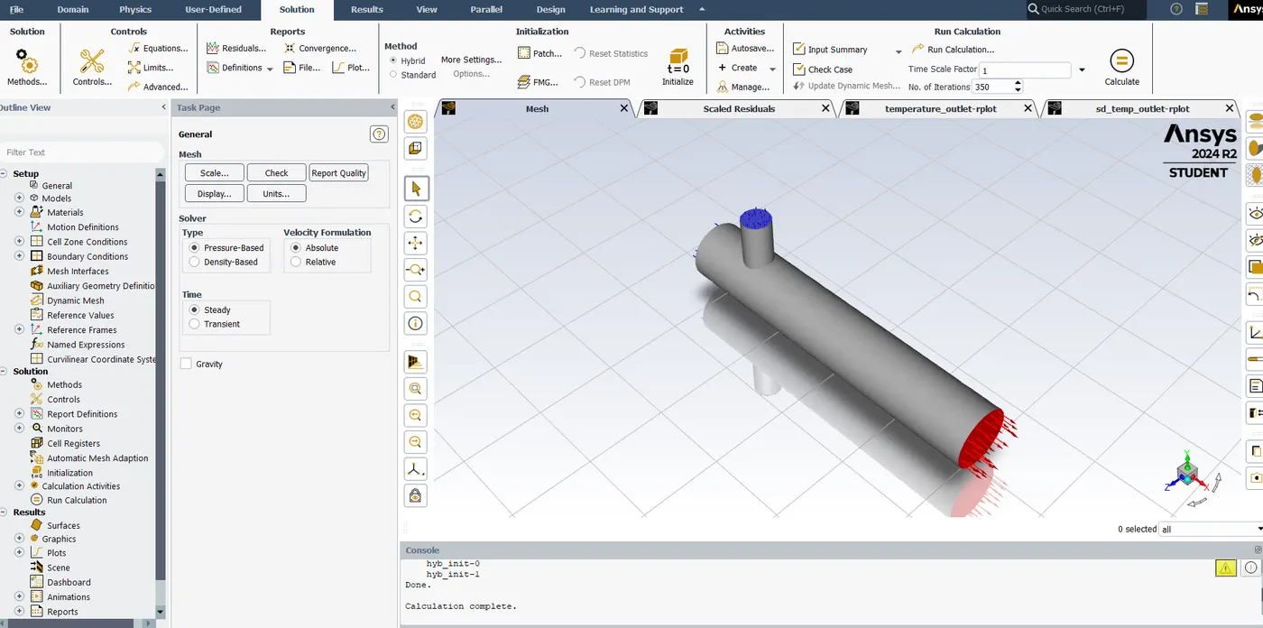
In all of these cases the geometry modifications are same. which are presented below.

1.Geometry loading into workbench

-short Tee

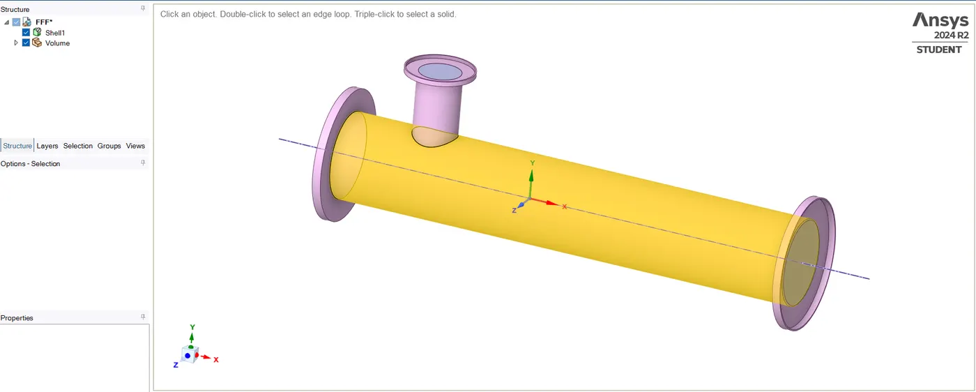
Once we load the geometry into any of the geometry module(Discovery, Space claim...), in the prepare select the volume extract to extract the volume which is not needed for the present calculations. After the volume is extracted from the side tree shell1 is suppressed and also from physical calculation using suppress physics option.

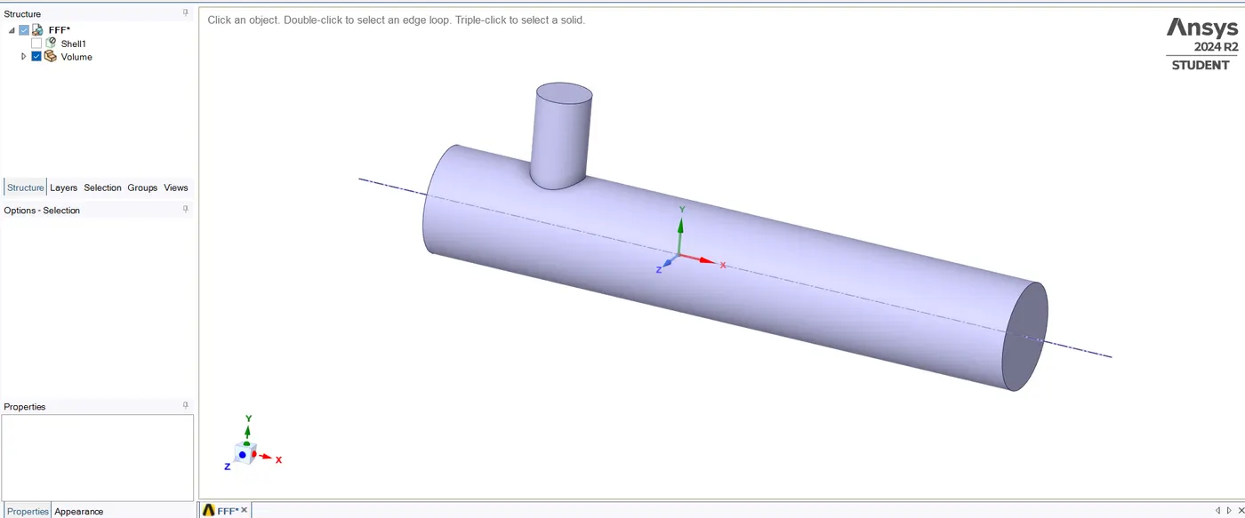
Similarlly long Tee

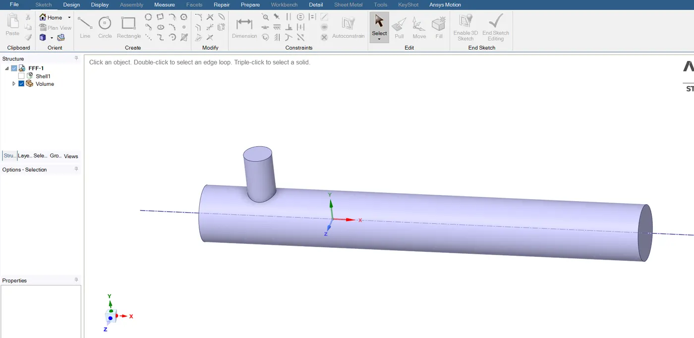
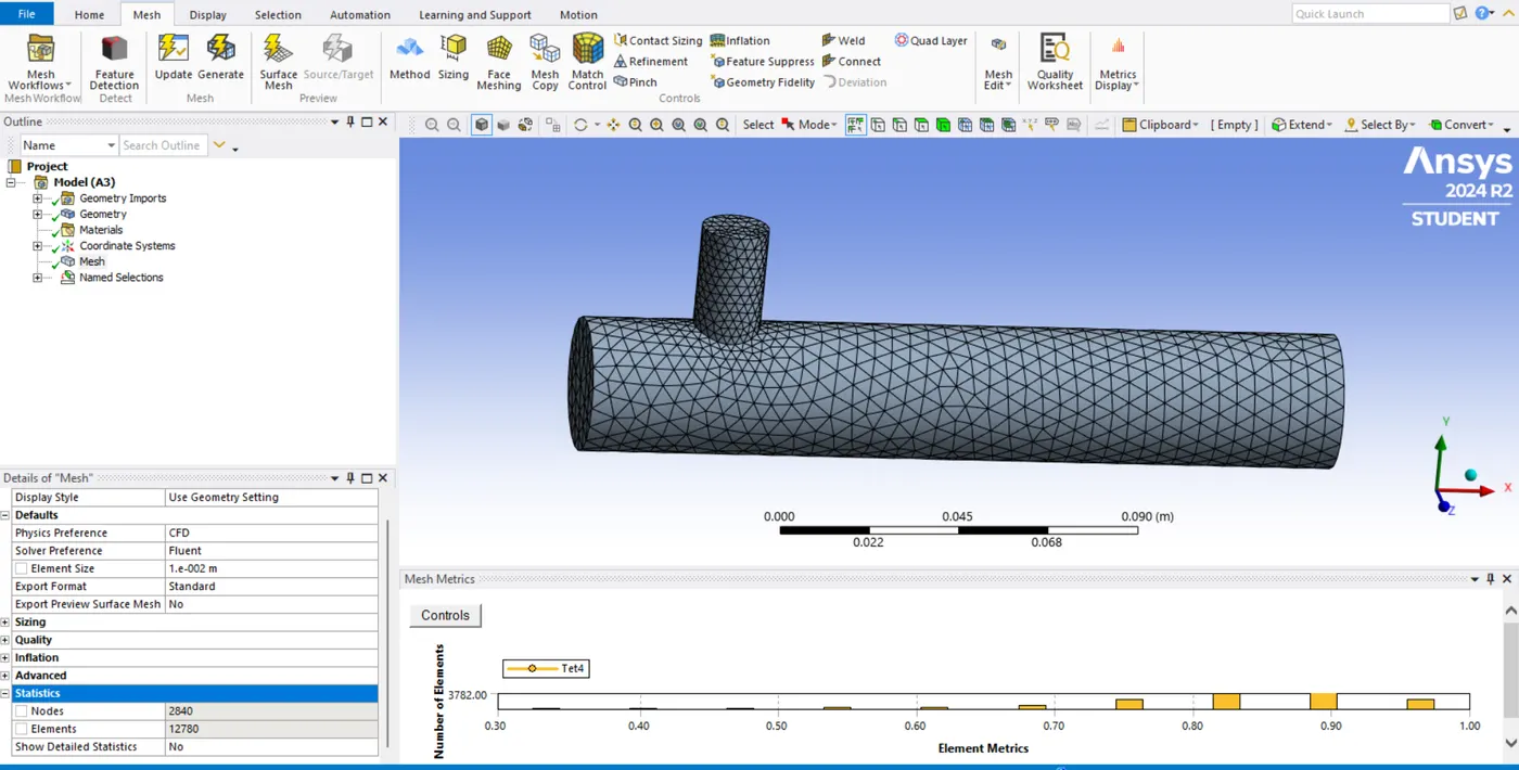
2. Meshing

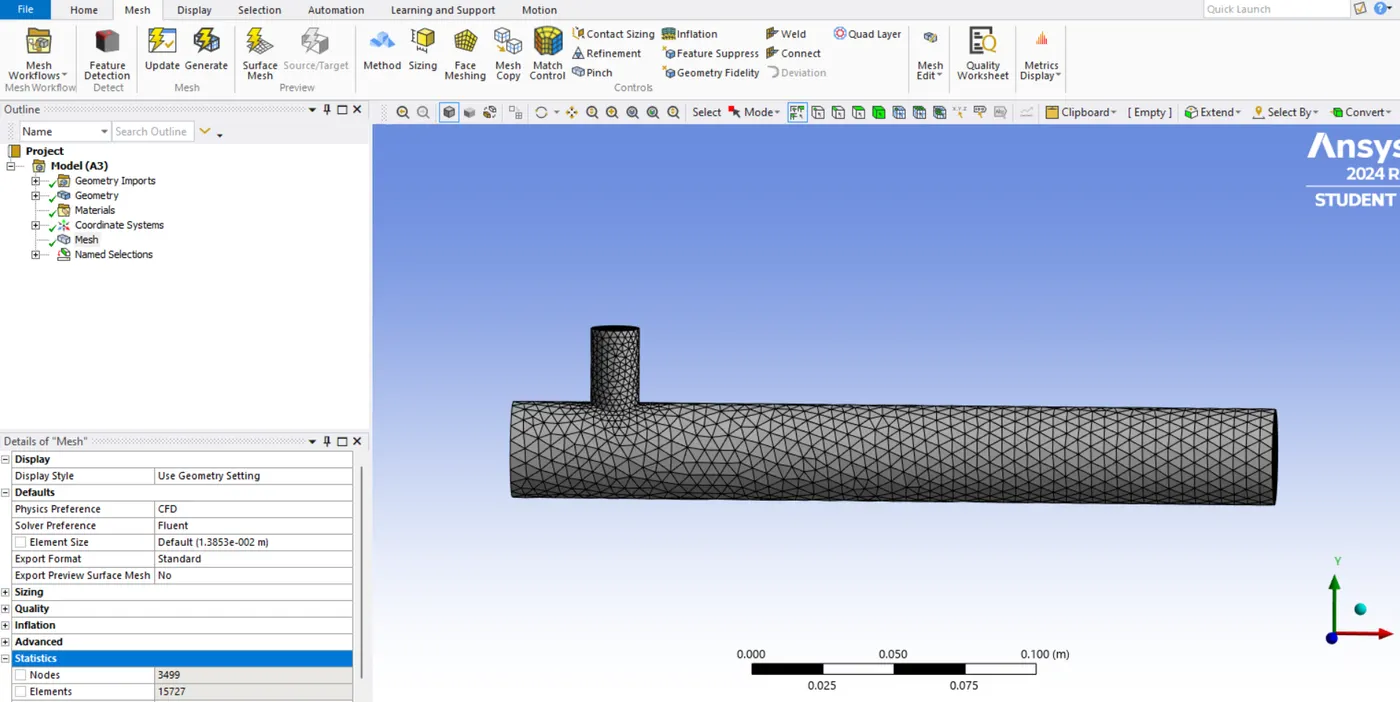
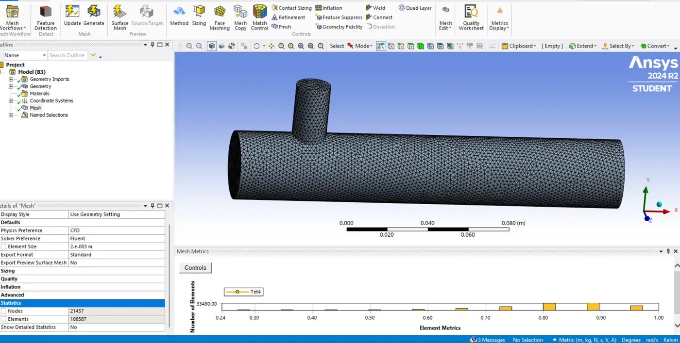
after finishing the geometry modifications, meshing is initialized. click on the mesh option in the left side tree and generate default mesh.The default size of the mesh is 1e-002

Similarly long Tee

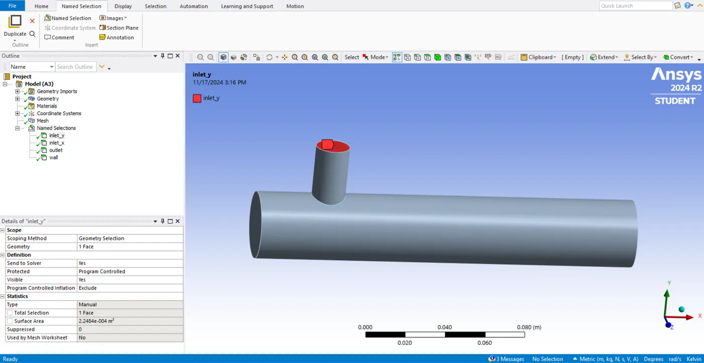
now select the surface option and create named selections for inlet_x, inlet_y, wall and outlet.

3. Problem setup

After the mesh setup model will be moved to fluent environment with double precision and the number of processors selected. The first thing to be done is check mesh quality with perform mesh check option.

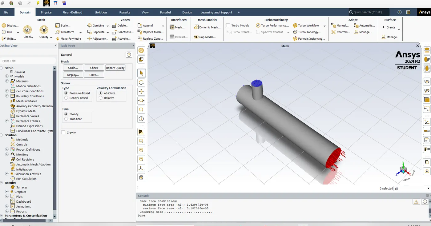
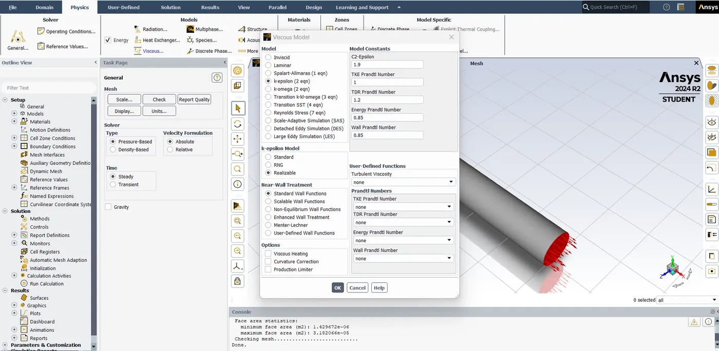
After the check, solver settings are selected. Pressure based, absolute velocity formulation and steady state solver. In the physics energy equation is activated with viscous effects to select the appropriate model. In the first try k-e model with realizable model is selected.

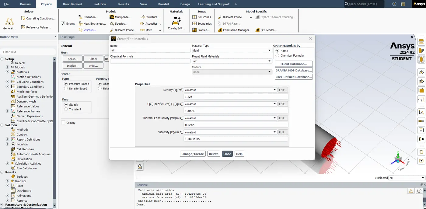
After this from materials create/edit materials if the material is air then ok. if the simulation need another material the changes need to be done here.

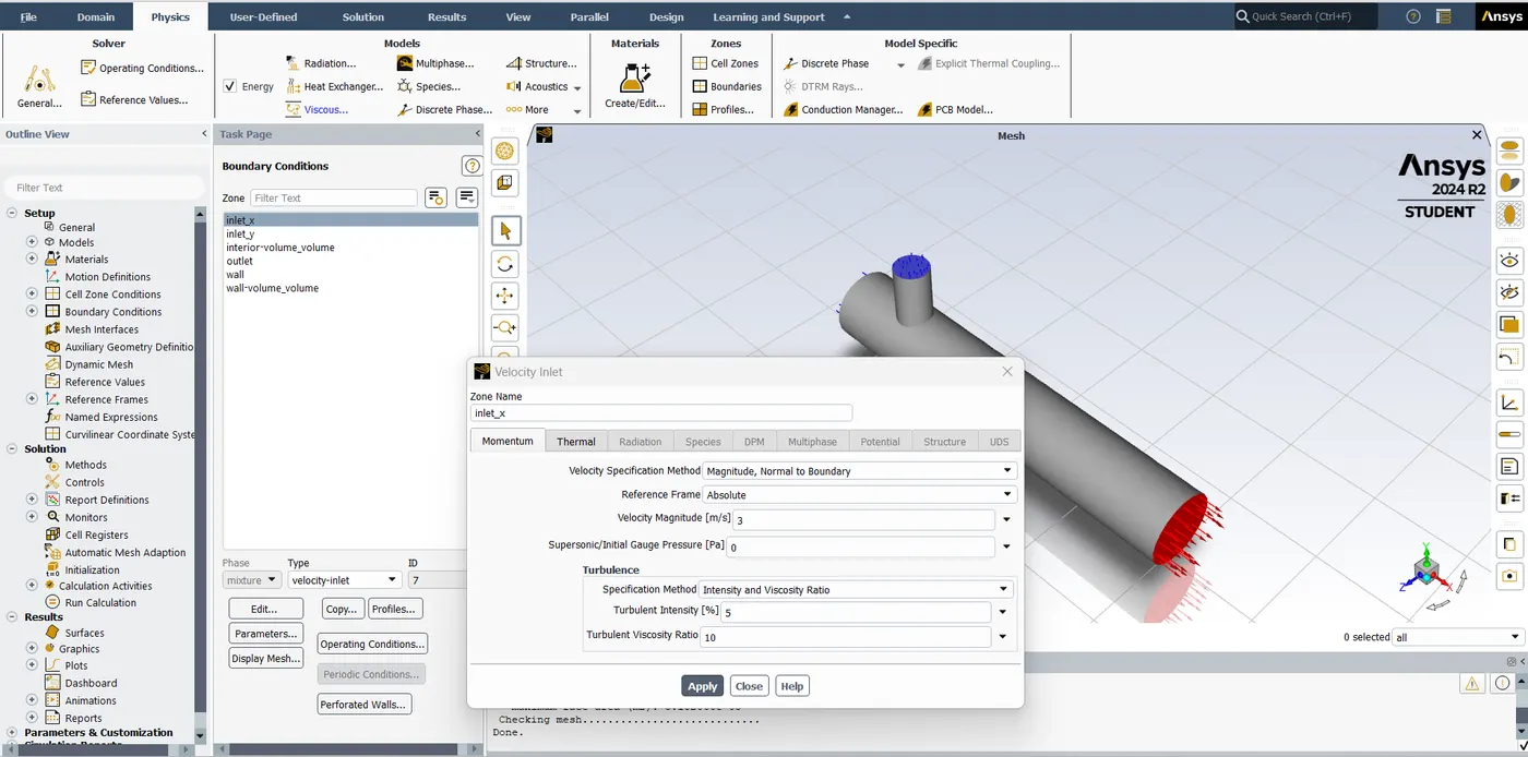
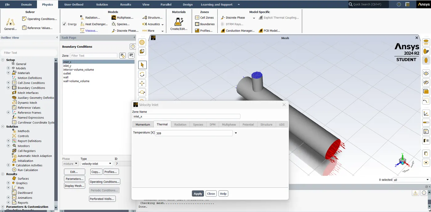
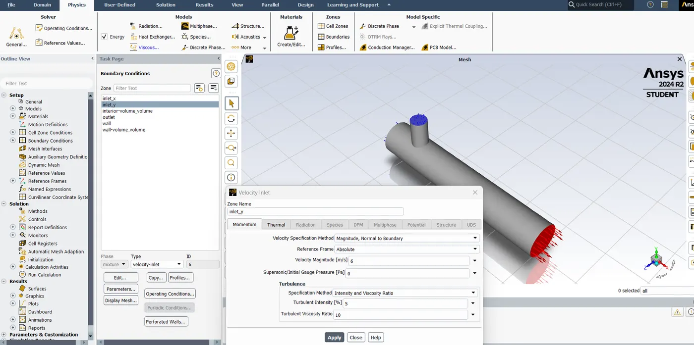
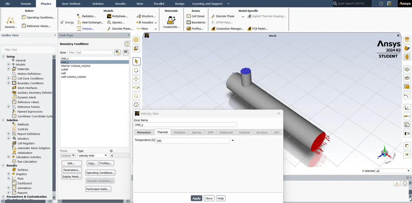
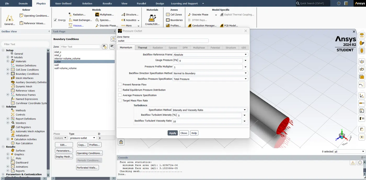
After the materials, boundaries are selected from the zones to input the boundary conditions. From the calculation of momentum ration 2 inlet_x velocity being 3 m/s. inlet_y velocity will be 6 m/s and the outlet gauge pressure is 0. All of these conditions are edited in the boundaries.

inlet_y

outlet:

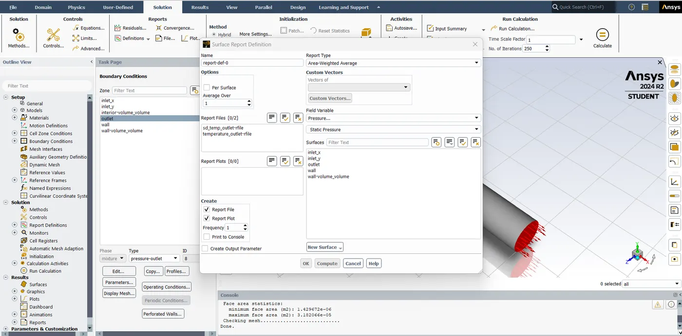
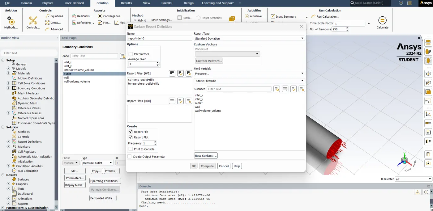
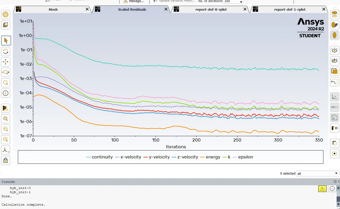
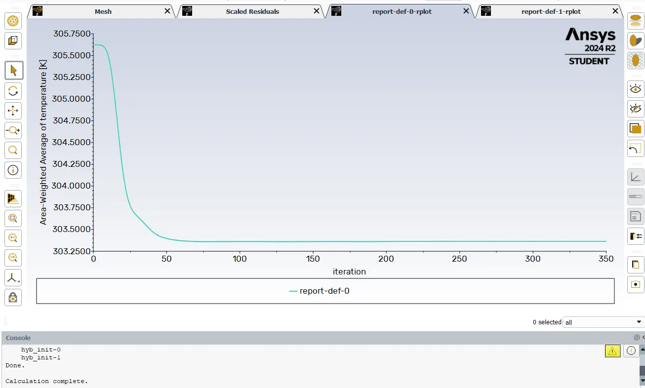
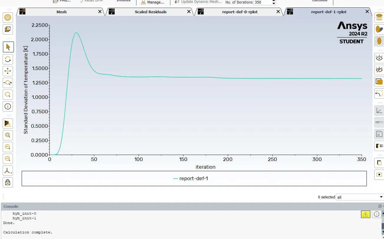
now after all the conditions. Now in the solution go to the definitions to create reports with area weighted avg of temperature and standard deviation of temperature which will be along with the residuals. After that initialization and enter the no.of iterations and run.

Initialization and calculation:

Results

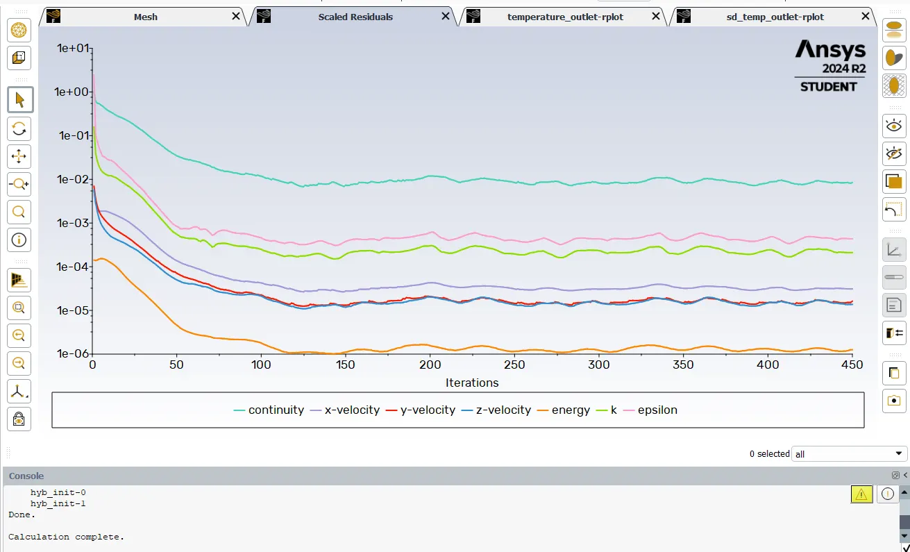
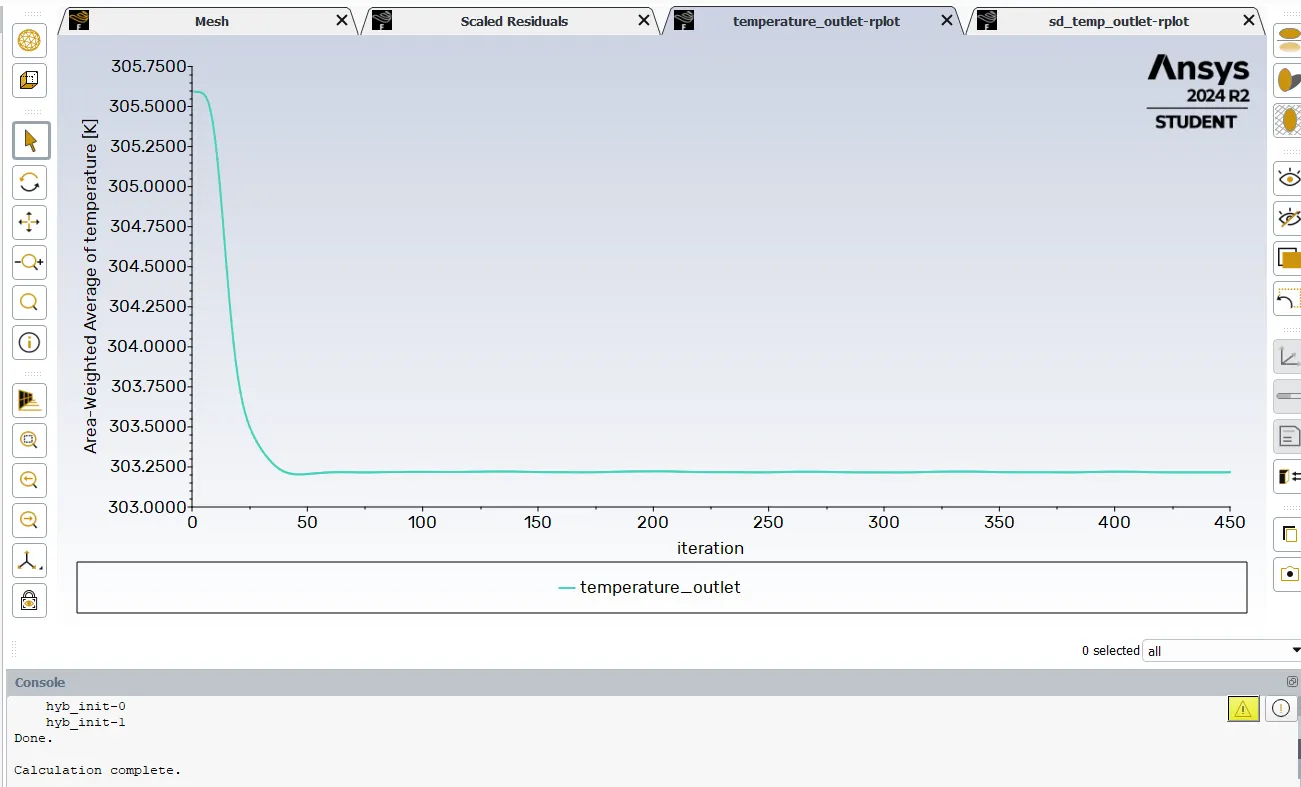
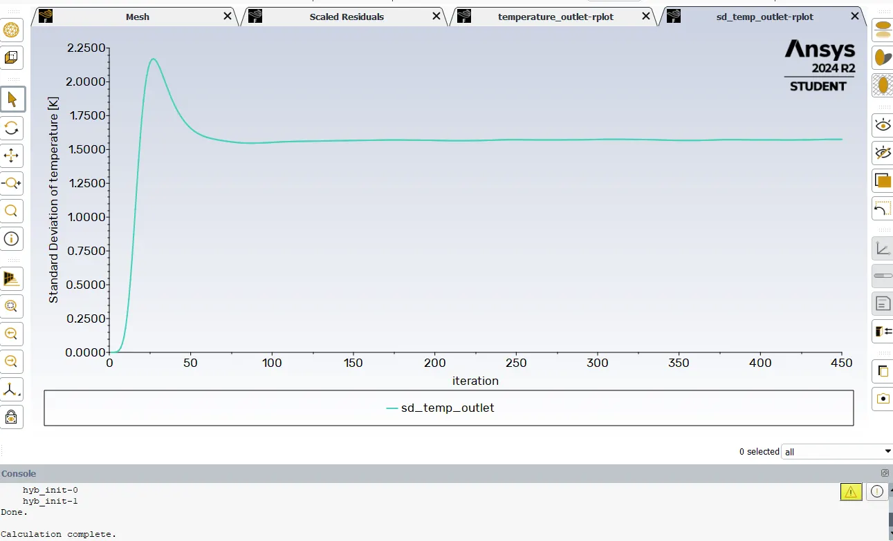
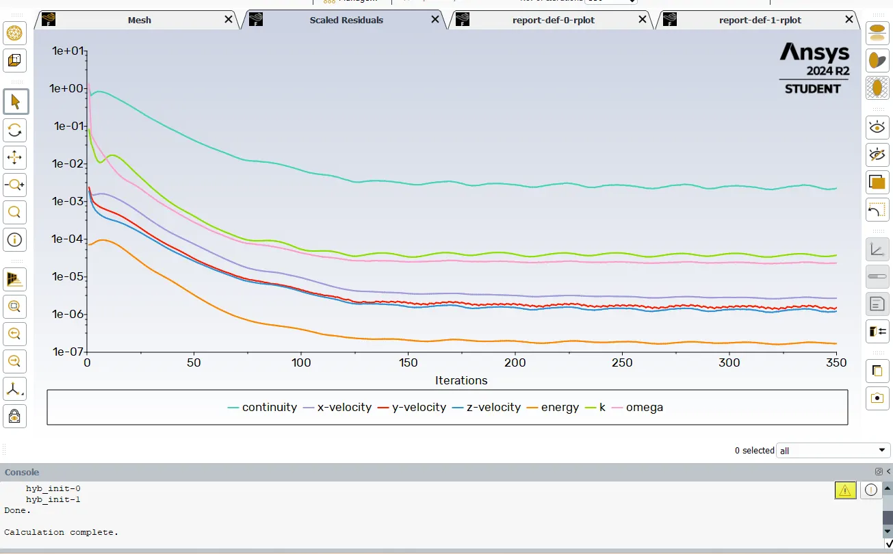
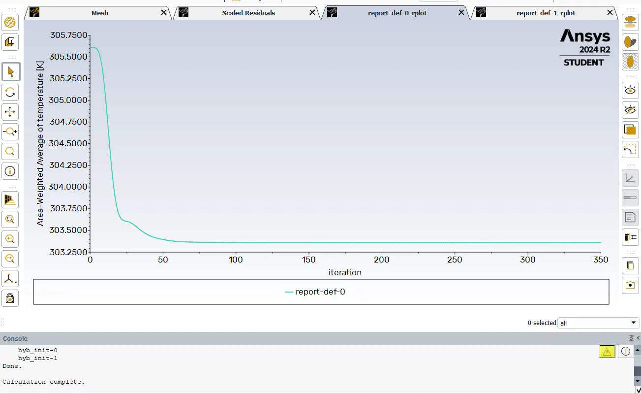
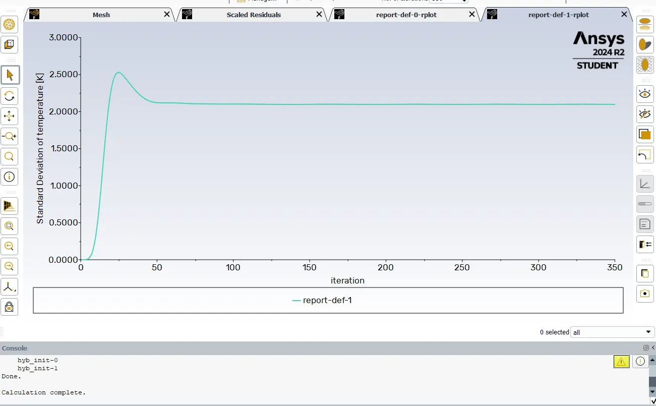
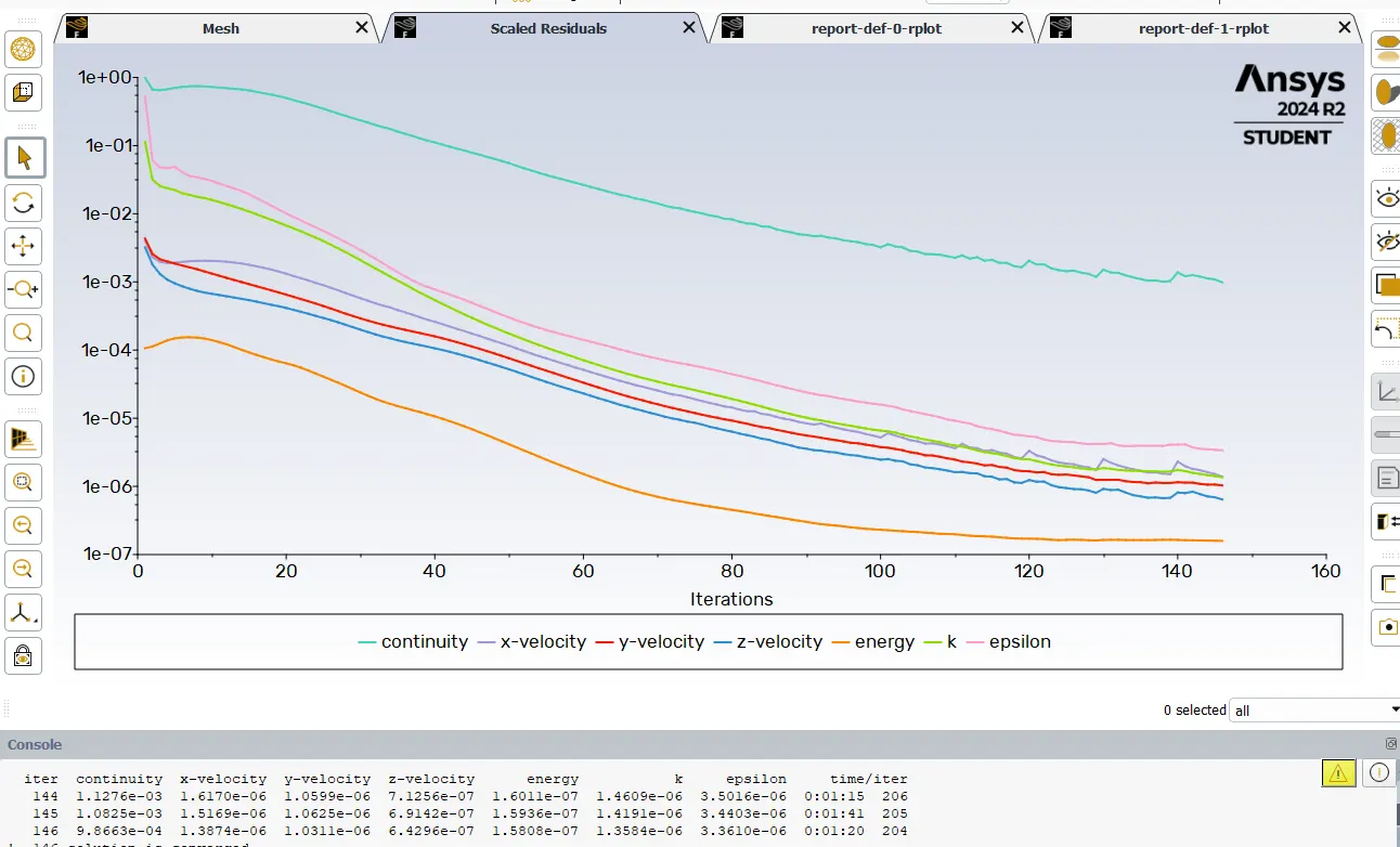
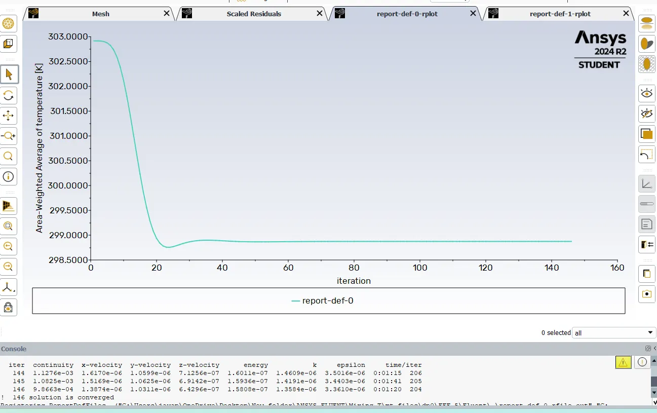
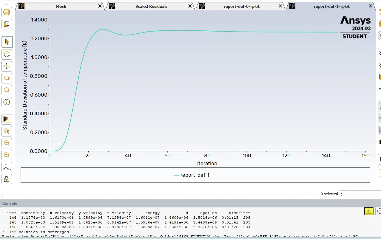
now that the solution is completed and converged as the residual values reach near 1e-03.The reports of temperature at the outlet area weighted average and standard deviation also become steady state around 75 iterations. Lets move to post processing to visualize the results.

Results for temperature and the velocity:

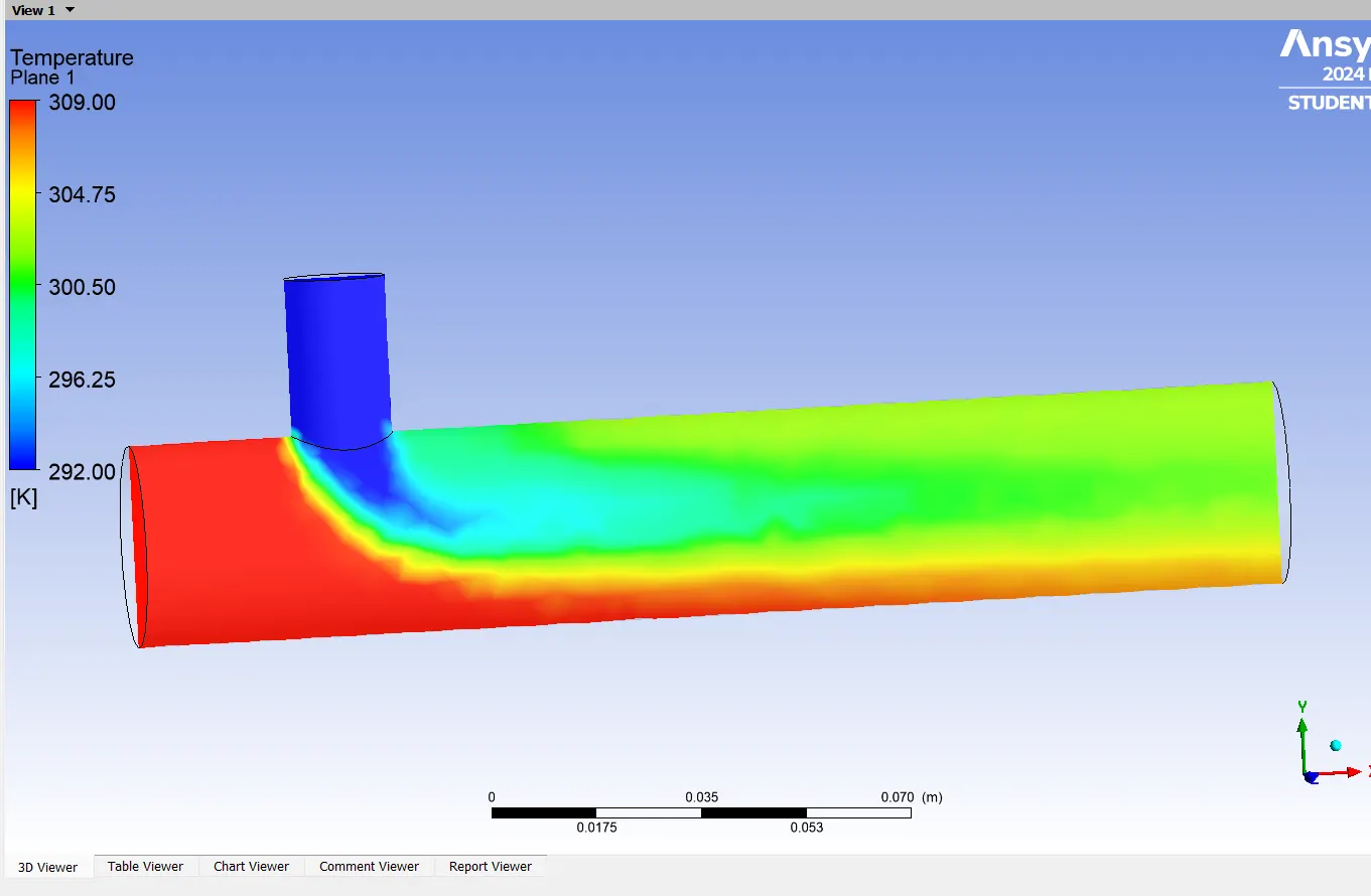
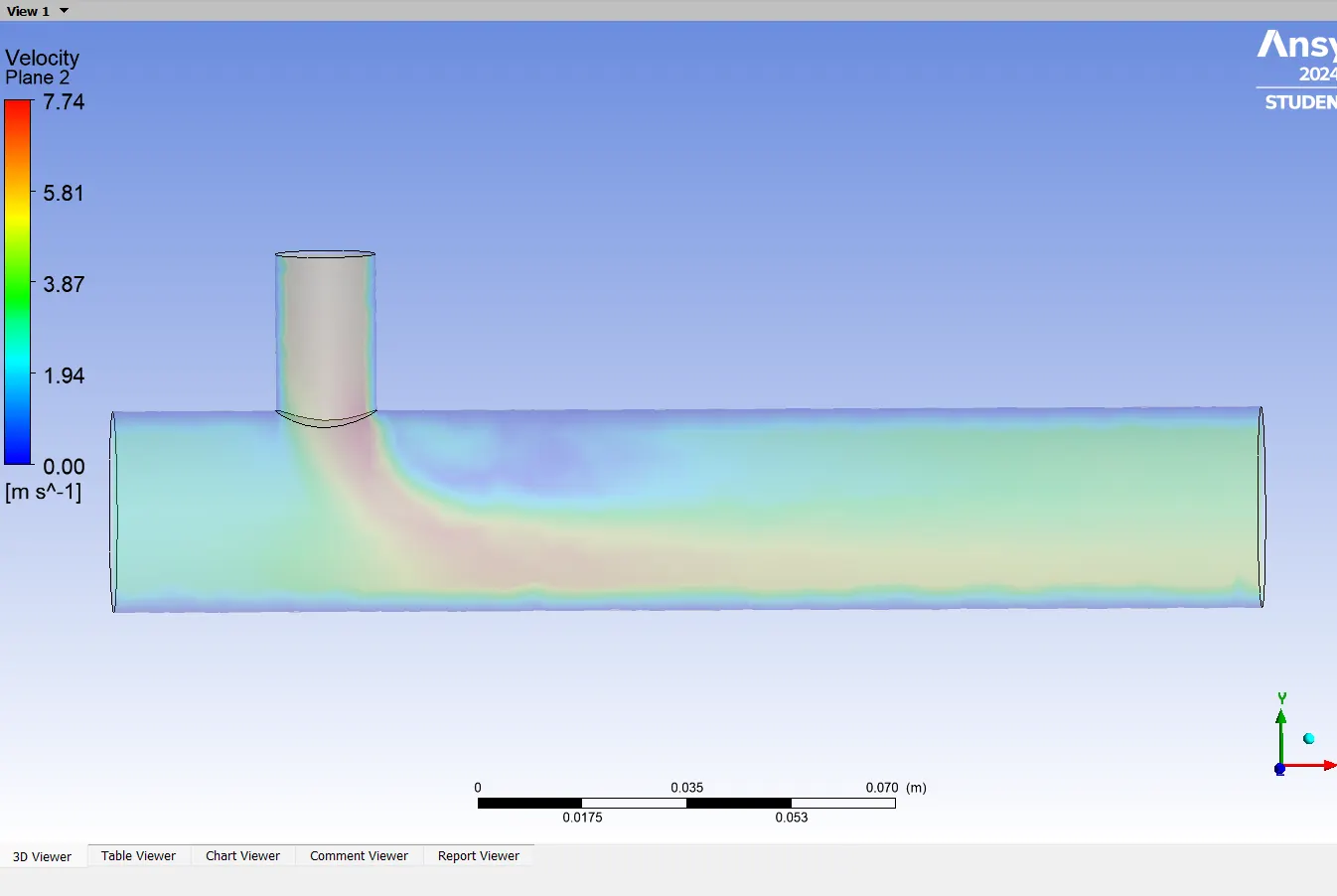
Now lets watch the results of the upgraded mesh set with the same model.

Mesh model with nodes and elements information with mesh size of 0.002.

Temperature plot:

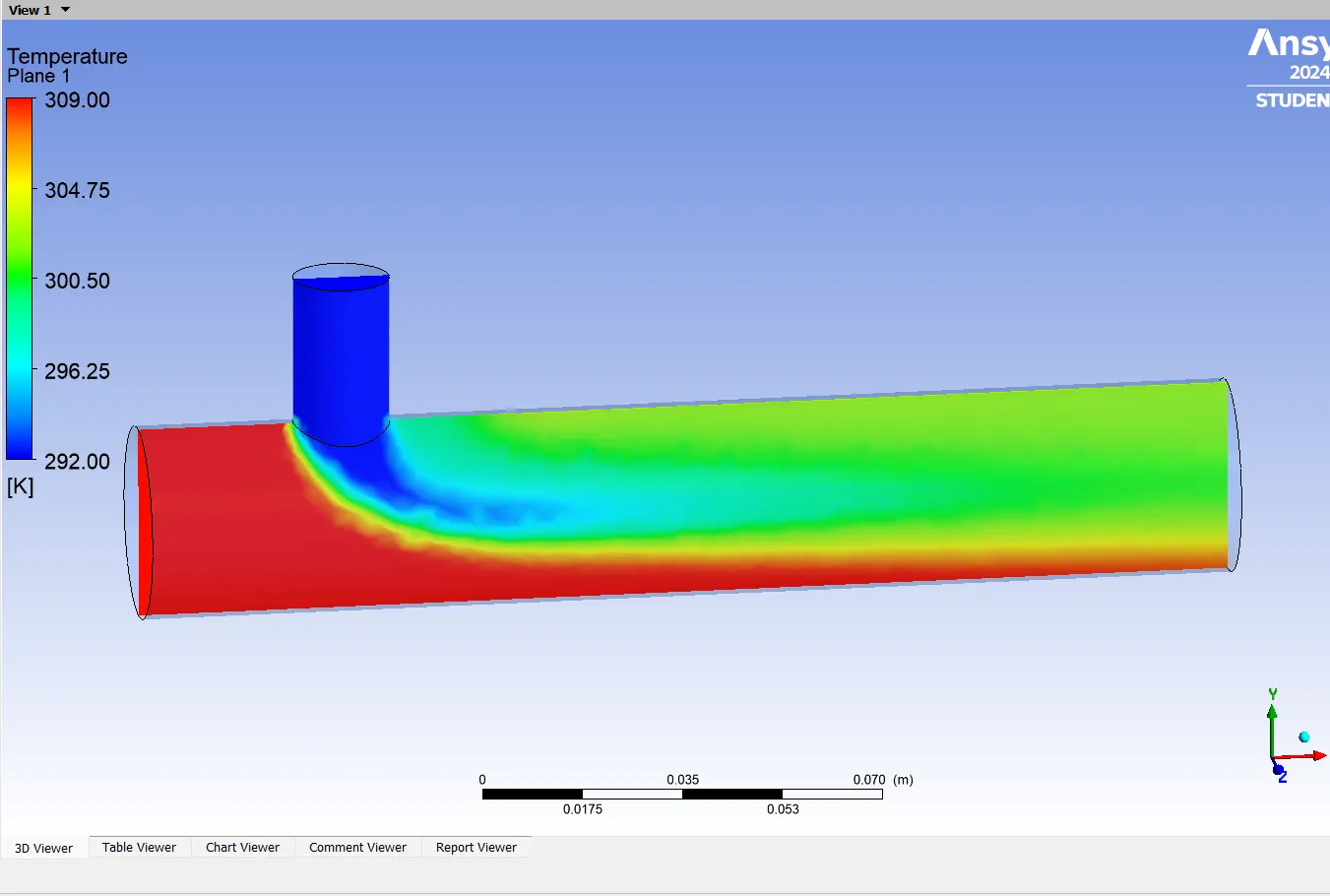
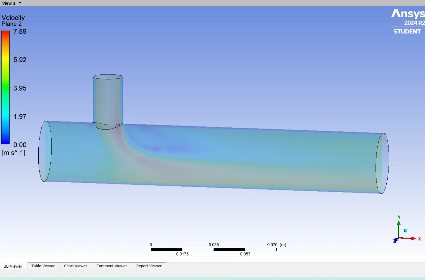
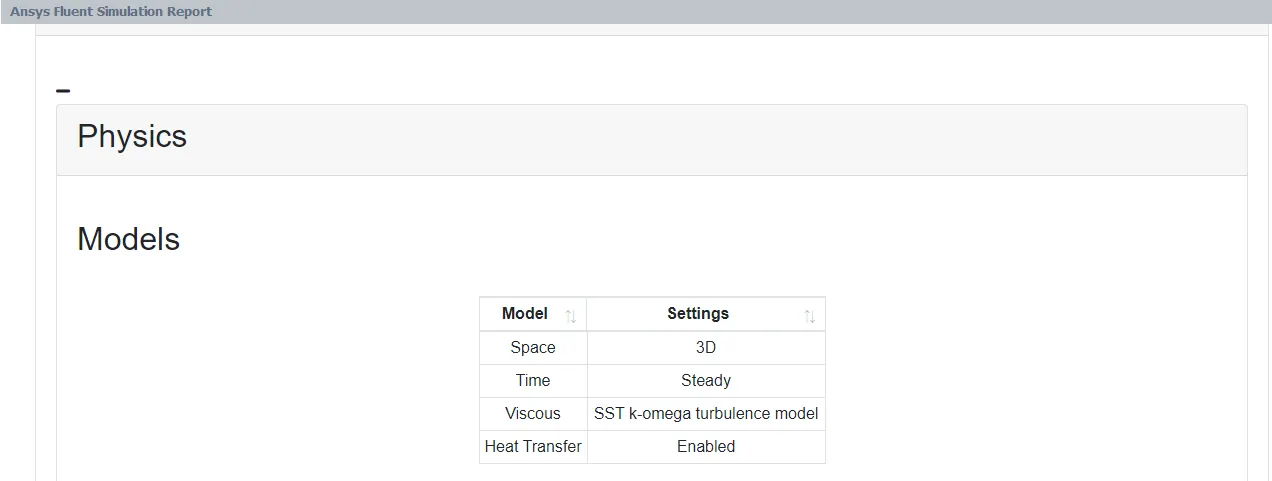
after looking at both of the temperature output results, finer mesh results in accurate results. so from now on the finer mesh is used for all of the simulations. now lets look at K-w SST model and compare with the results and choose a model for the next cases

Temperature & velocity plot:

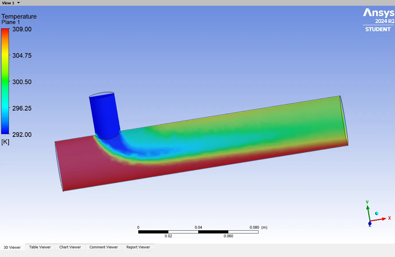
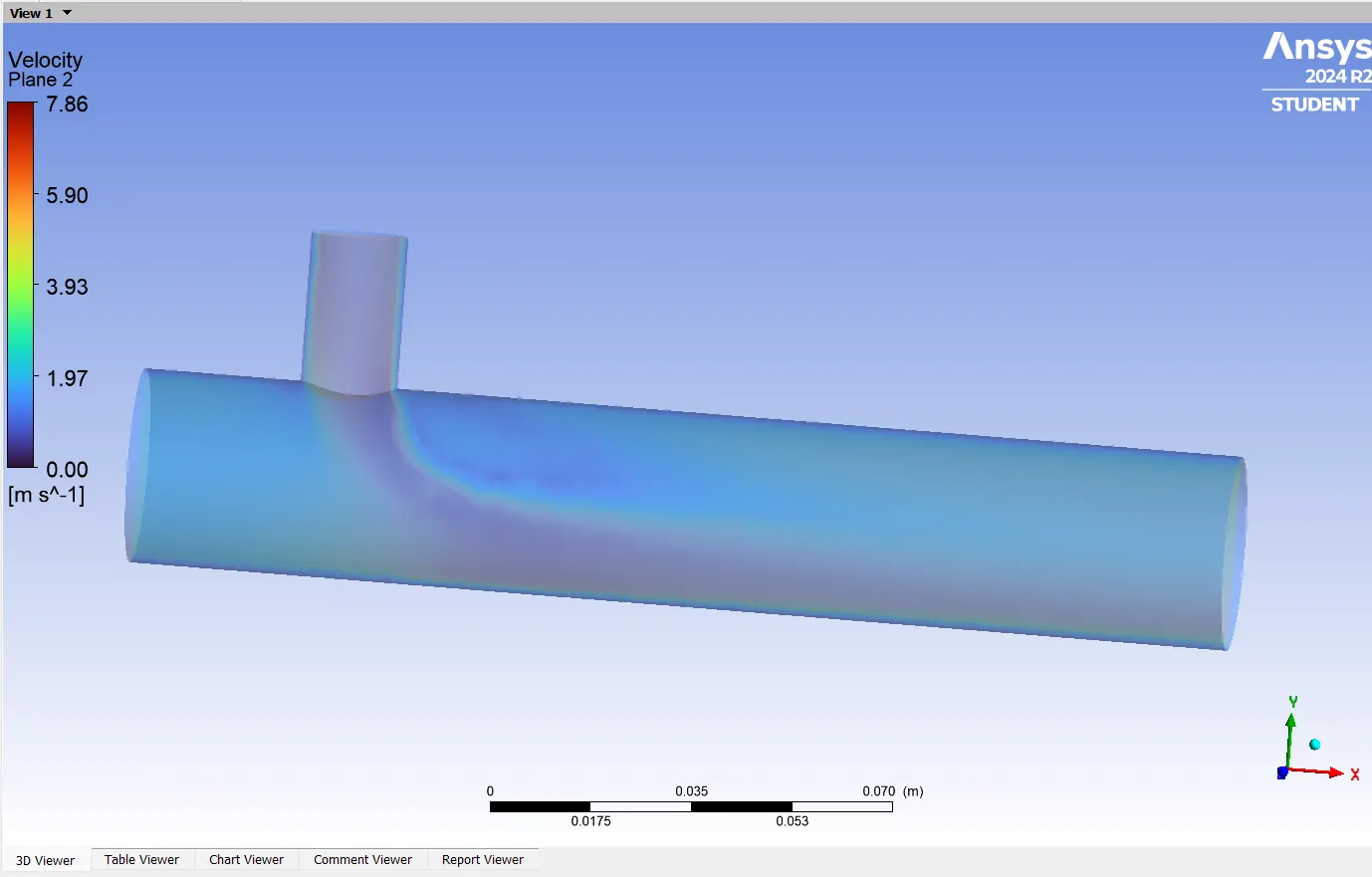
Based on the plots for temperature and the explanation of both the models in the earlier stage of the model explanation 𝑘−𝜖 model, 𝑘−𝜔 model, the 𝑘−𝜖 model is chosen for the further calculation.

The reason for this is 𝑘−𝜔 SST(shear stress transport model) is a type of 𝑘− 𝜔 model with near wall functions. In the present case we are interested in the mixing of the fluid so the 𝑘−𝜖 model is used further.

Case 1 (Short Tee) with MR=4:

Temperature & Velocity plot:

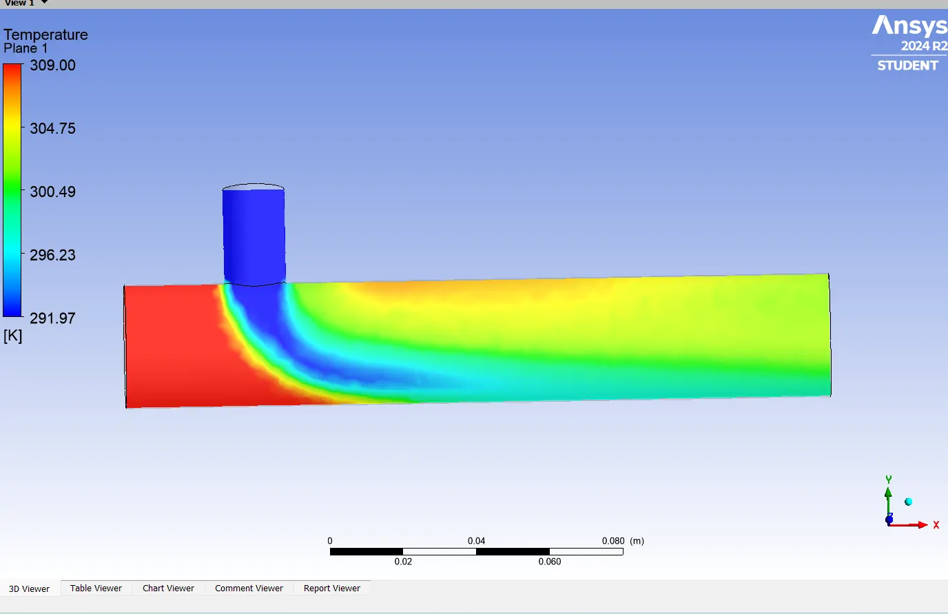
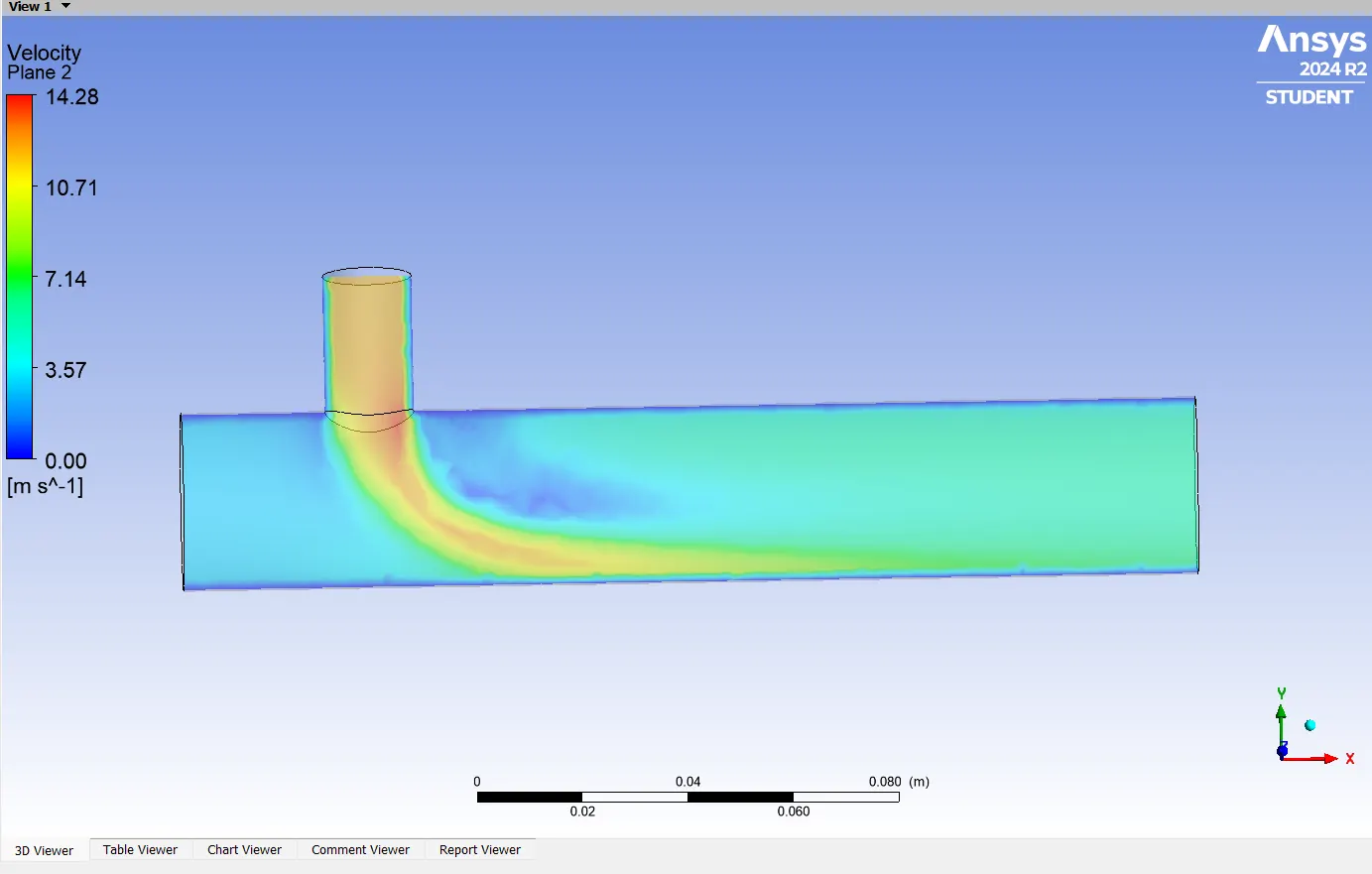
Based on observation between short pipe with MR=2 and MR=4,MR=4 has better mixing compared to MR=2.

Now lets move to long Tee with MR=2 and MR=4

MR=2:

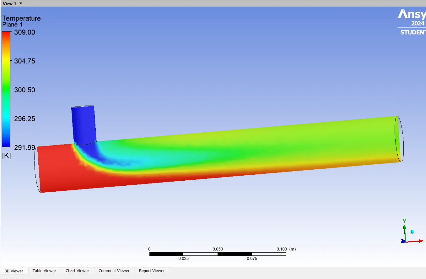
Temperature & Velocity Profile:

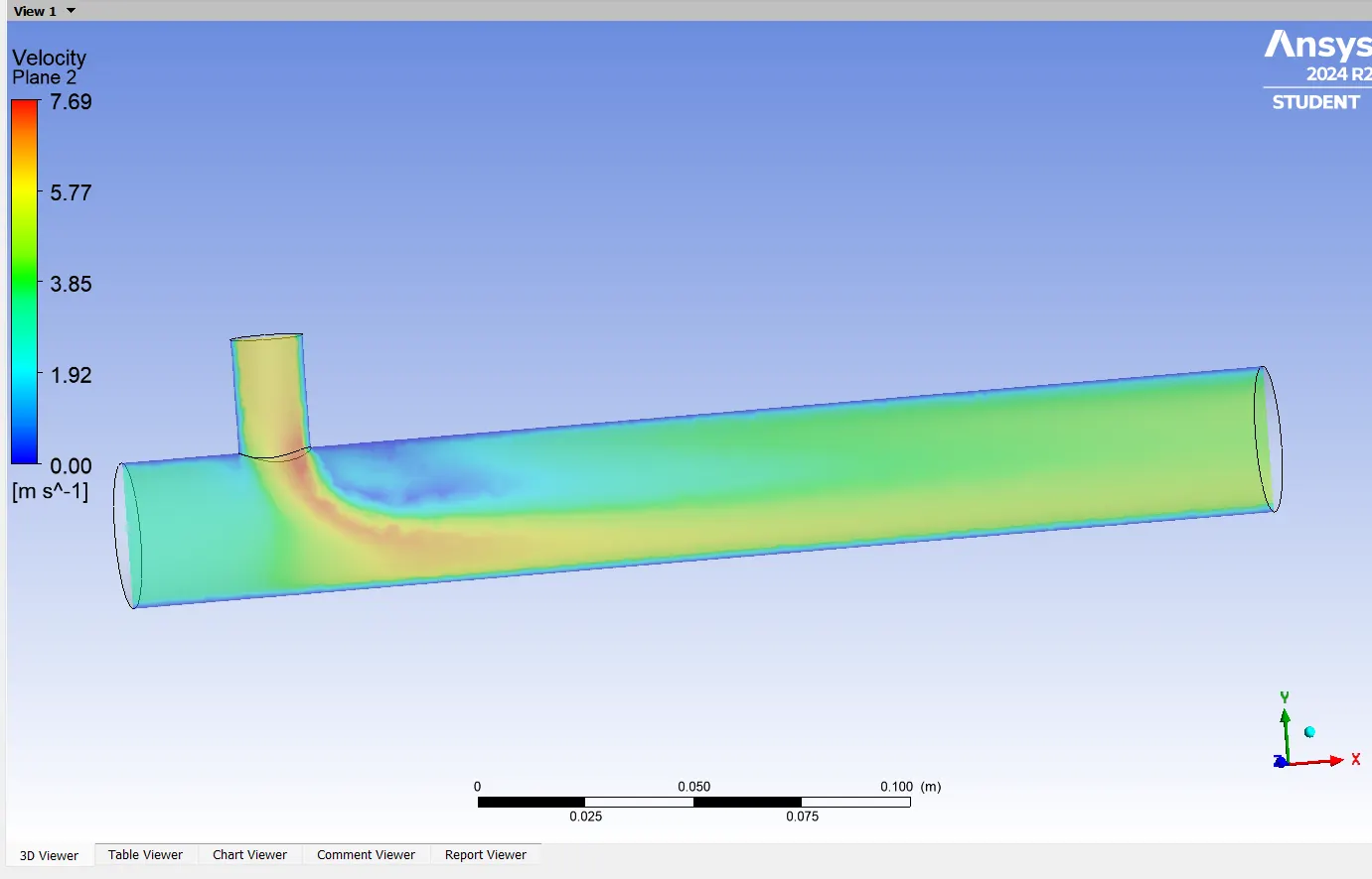
MR=4

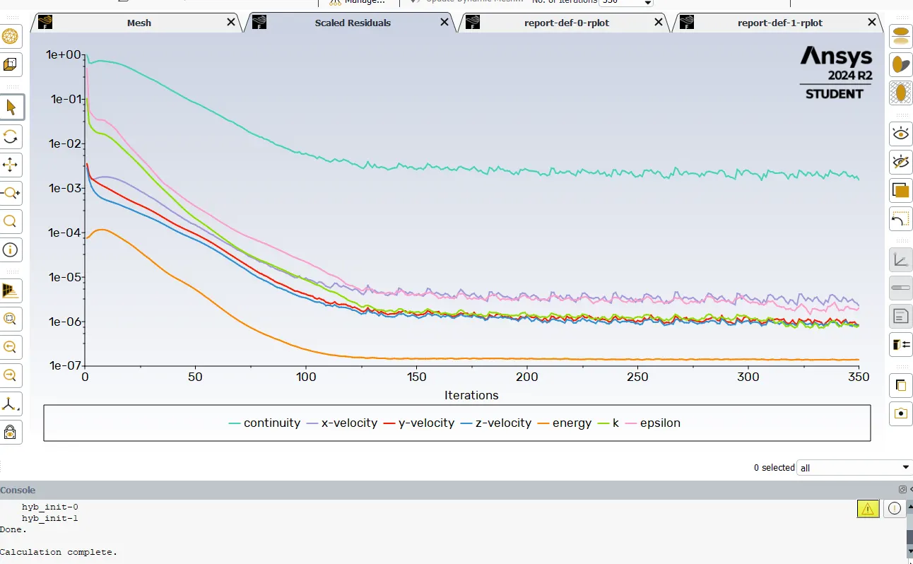
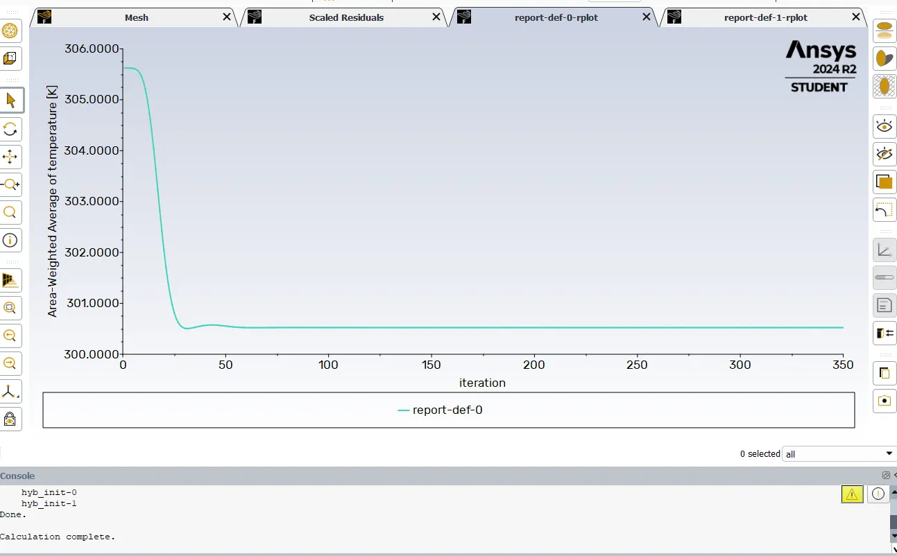
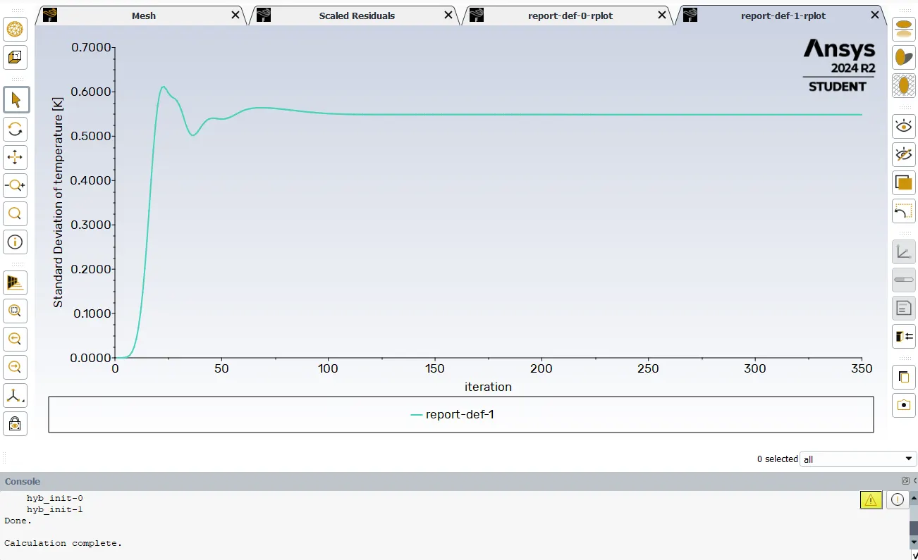
Temperature & Velocity Profile:

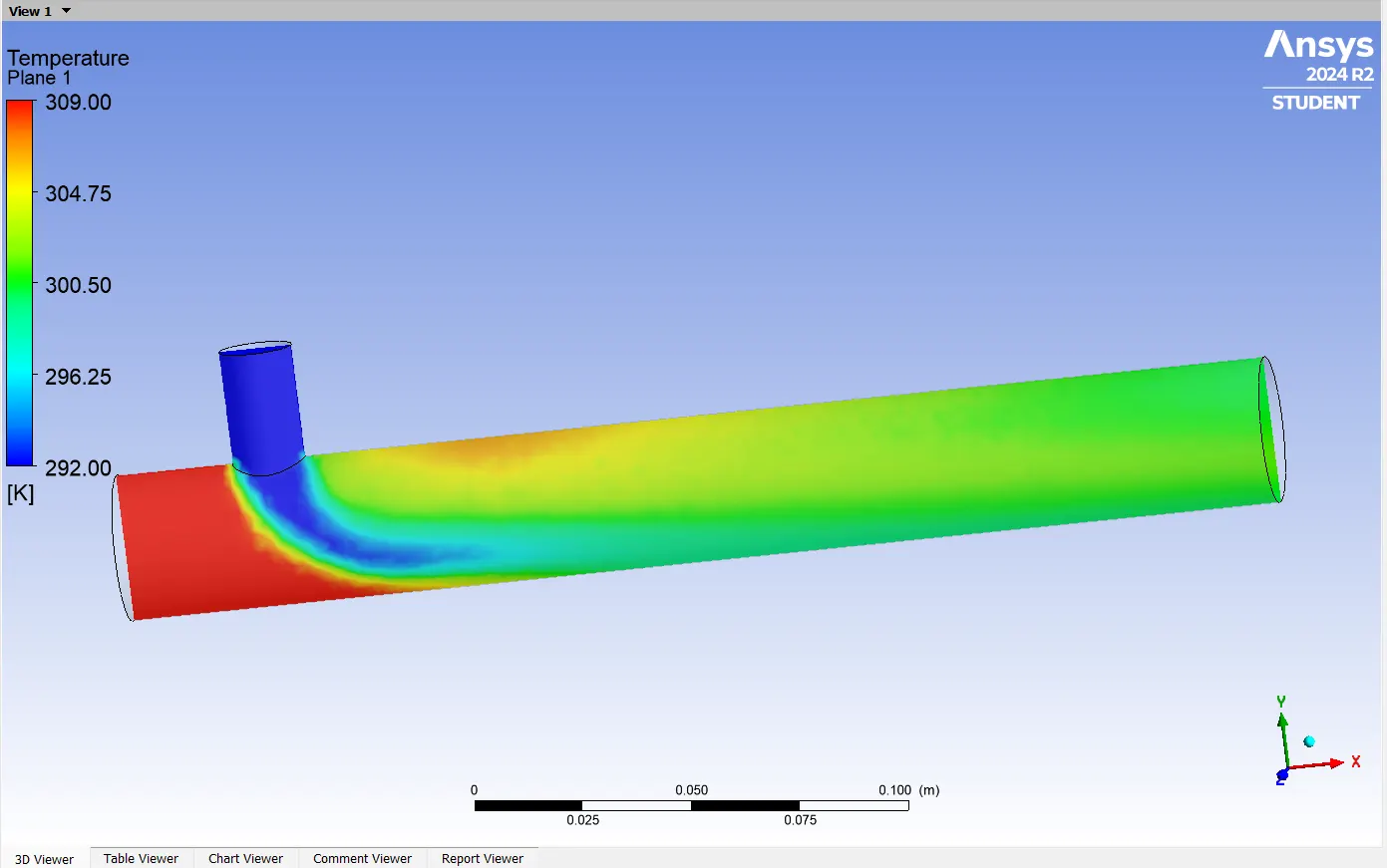
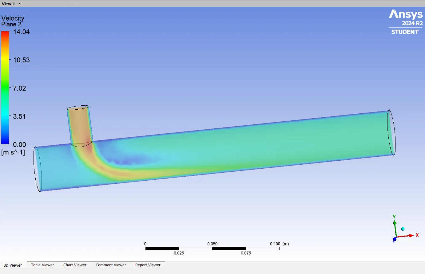
In the case of long Tee also the mixing is good in the Momentum ratio high case.

Type/parameter	cell count	Avg. outlet Temperature(K)	Iterations for convergence
Short Tee (MR=2)	61186	303.395	240
Short Tee (MR=4)	61186	300.578	225

Type/parameter	cell count	Avg. outlet Temperature(K)	iterations for convergence
Long Tee (MR=2)	86660	303.361	146
Long Tee (MR=4)	86660	300.523 168

Comparing the two models with respect to length did not make that much of change in the results whereas the momentum ratio make much difference in mixing. When the momentum ratio is higher we can expect a good mixing.