Week 1- Mixing Tee
Aim: To model mixing Tee using 2 different SST models in ANSYS
Introduction: Mixing Tee is where two pipes are joined at right angles to each other. It is a cost-effective way to perform mixing of 2 fluids. It is used in chemical reactors to combine reactors. Used to mix cold and hot water streams to achieve desired water temperature. To combine different temperature streams of feed water before entering the boiler to ensure uniform temperature and to avoid thermal shock
Theory: Mixing Tee results in a uniform temperature distribution in the outlet, if the outlet is long enough. The resulting temperature can be calculated through the given formula. The mass flow rate can be replaced with velocity as density and area are considered constant throughout the experiment.
Tmix =303.33K = 30.330C
Solving and Modelling approach: The short Tee geometry is solved using 2 solvers k epsilon and k omega. The standard deviation of outlet temperature and the residual is calculated as graphs. The best model is chosen and implemented in the long Tee geometry.
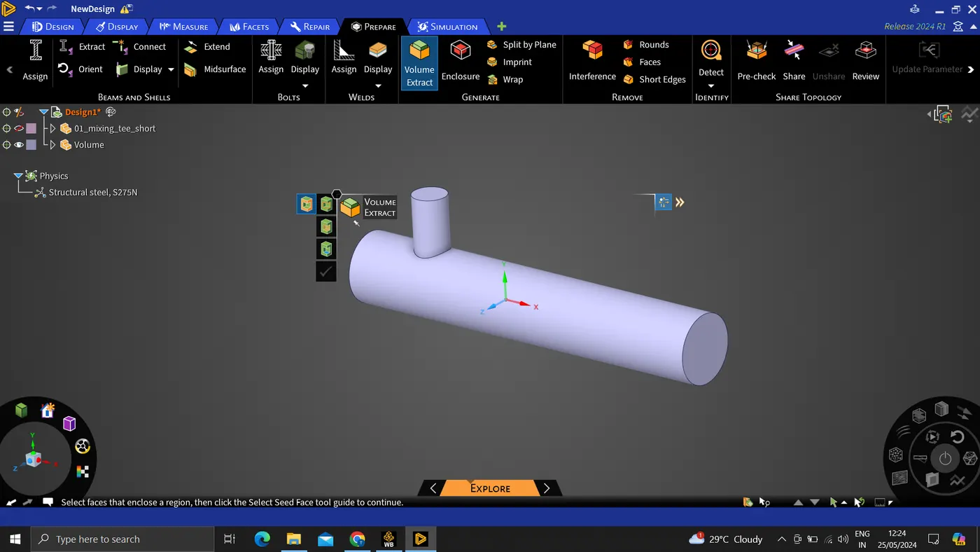
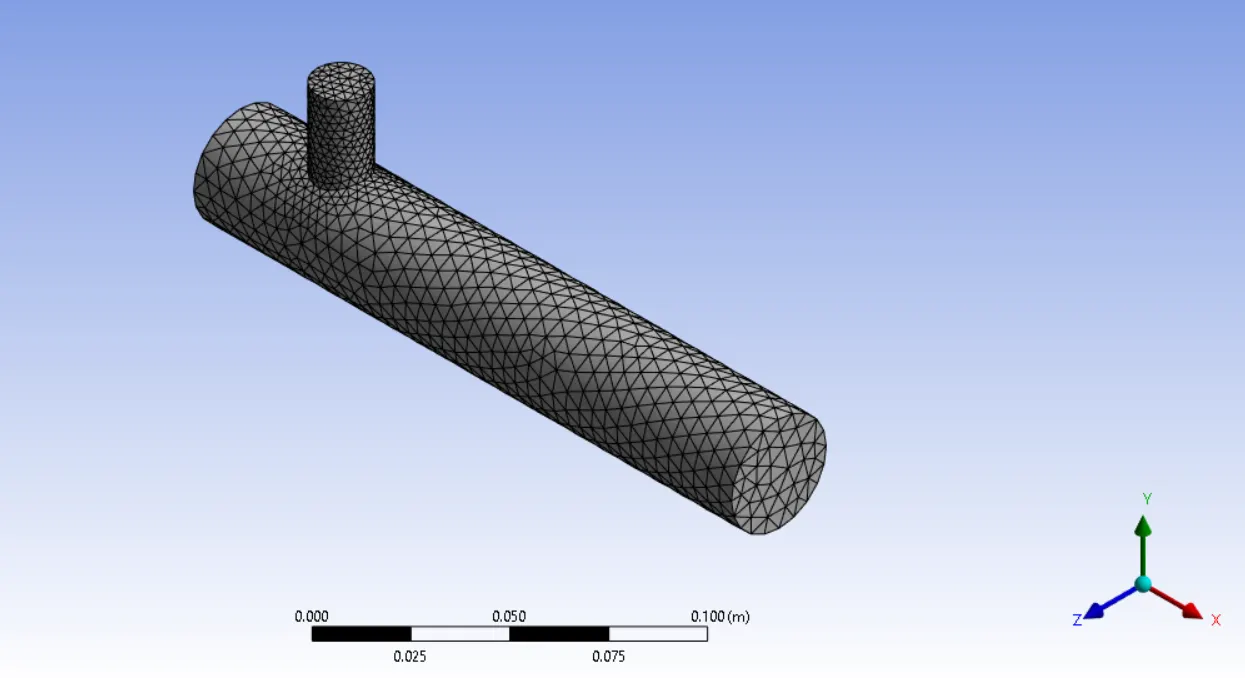
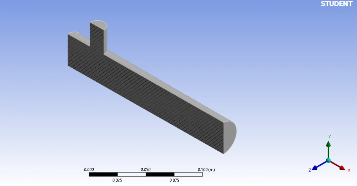
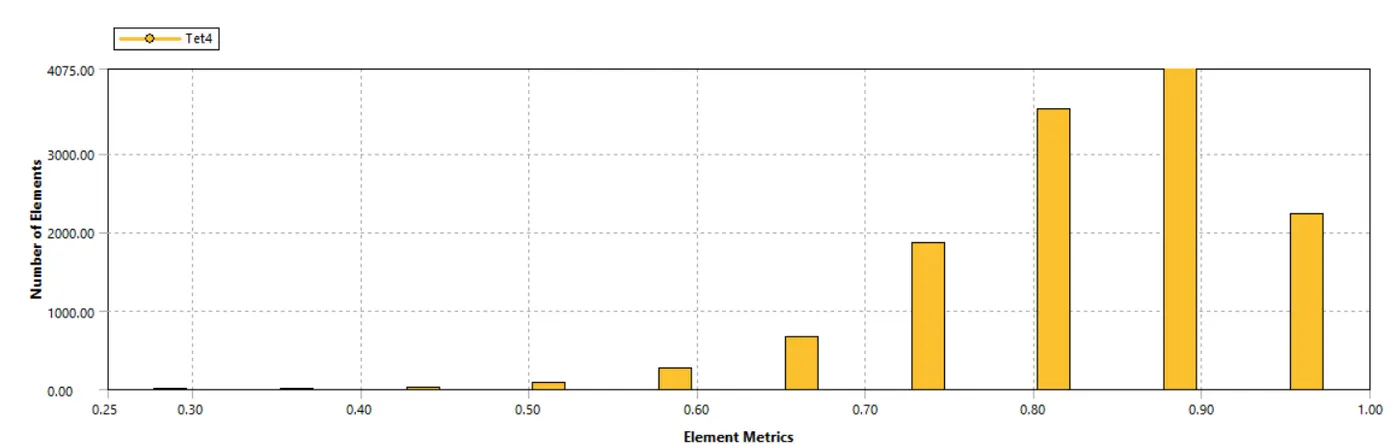
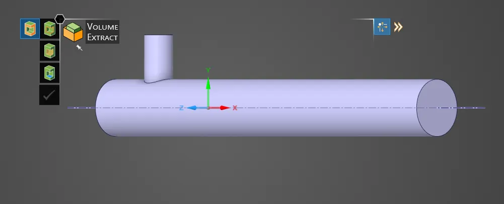
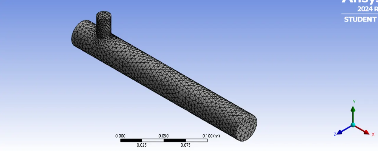
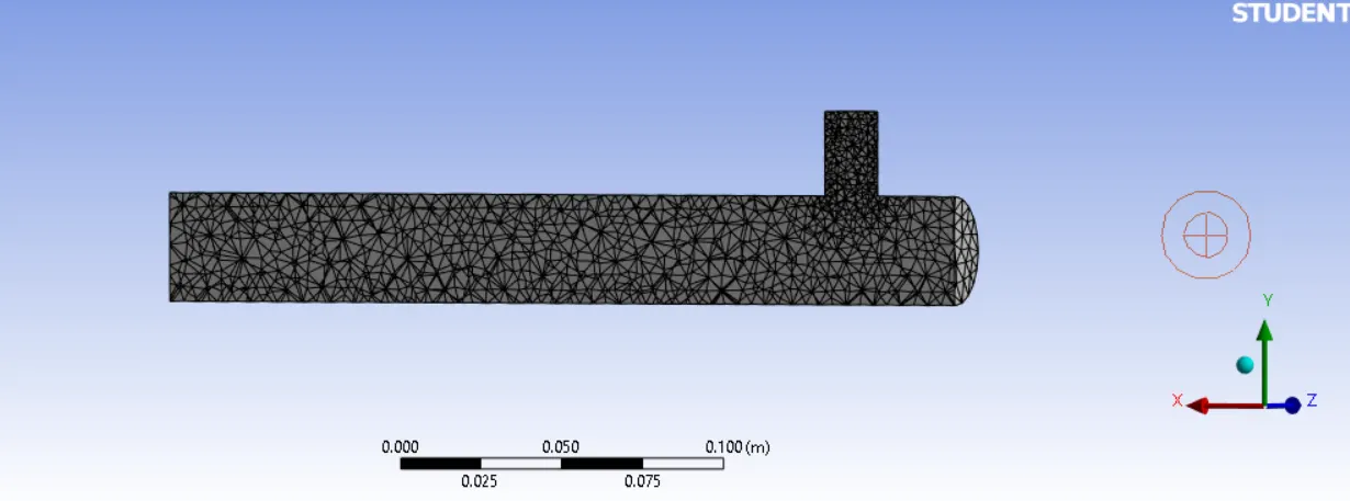
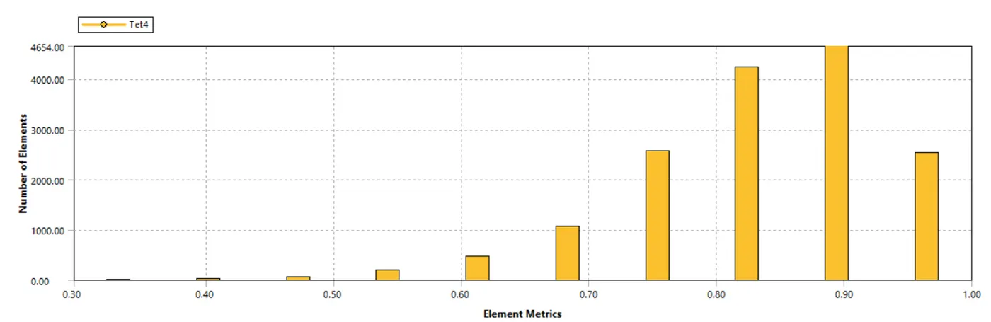
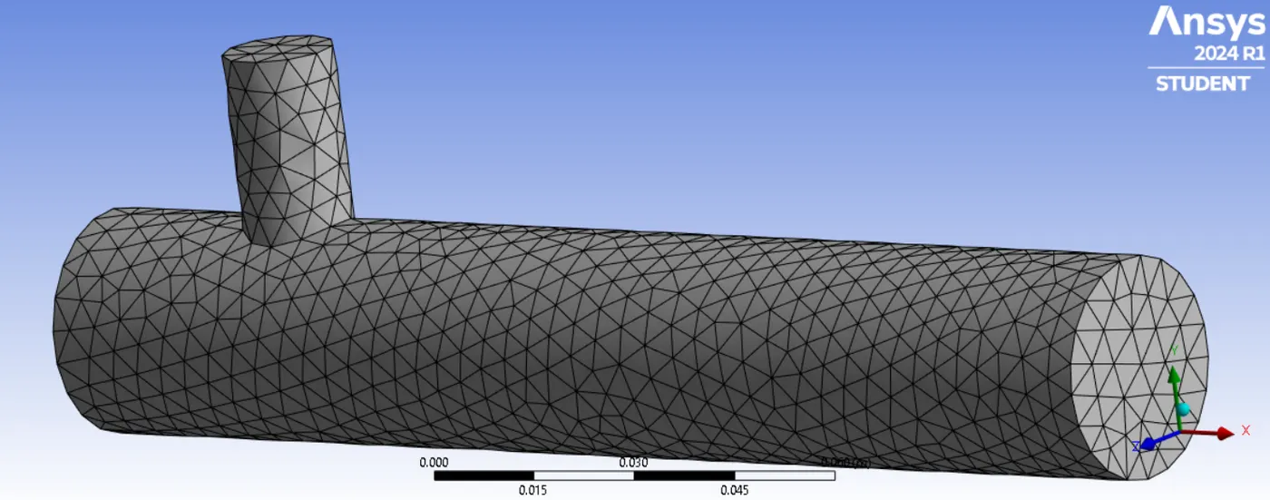
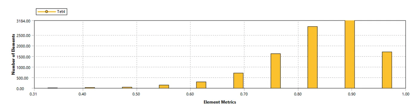
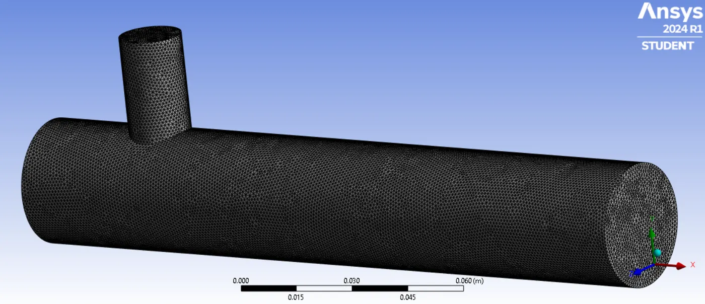
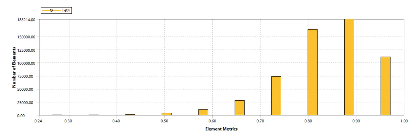
Short Tee geometry is imported into the Ansys DISCOVERY. The volume is extracted from the geometry using the edges option. The rest of the geometry is excluded from the simulation. In the mesh window named selections are made. Element size is set to default(1.0219*e-2m). Mesh metric element quality is given. Mesh is generated. A section plane is created to view the mesh properly.
In the CFD solver, 12732 tetrahedral cells are created for short Tee. The solver is double precision, solver process 4. Mesh quality is checked. In pressure-based solver type, Steady solver time and absolute solver velocity formulation are chosen. Energy, viscous k epsilon model is chosen first and duplicated as k omega solver for the next case. For the k epsilon model standard wall function is given with near wall treatment. According to the THZ test case in the research paper, the material is water. In boundaries inlet and outlet velocities and temperatures are given. Outlet gauge pressure is zero. In the solution definition, the area-weighted average and standard deviation of the outlet is created. The solver is initialized in hybrid mode and runs for 150 iterations. Then calculate.
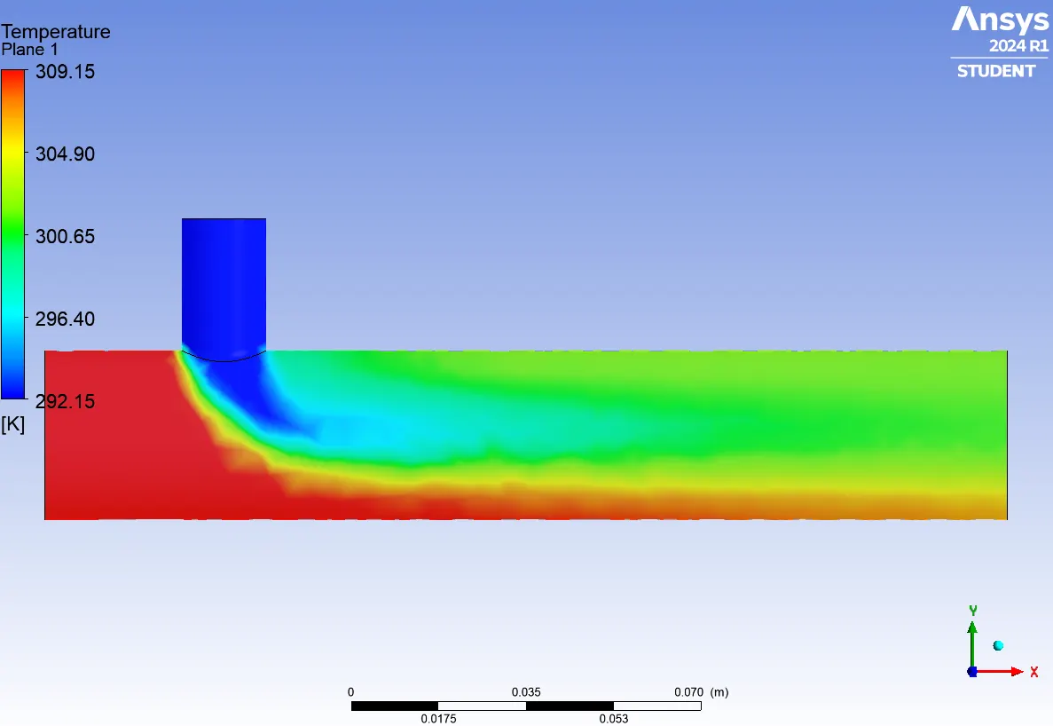
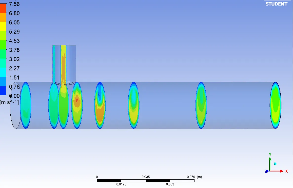
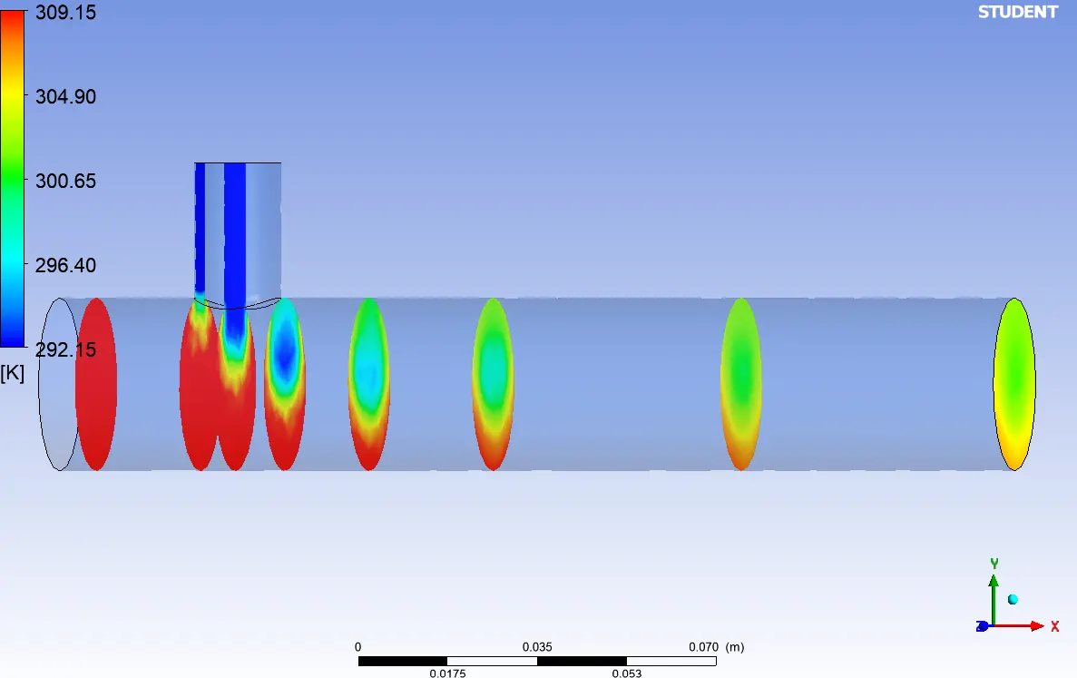
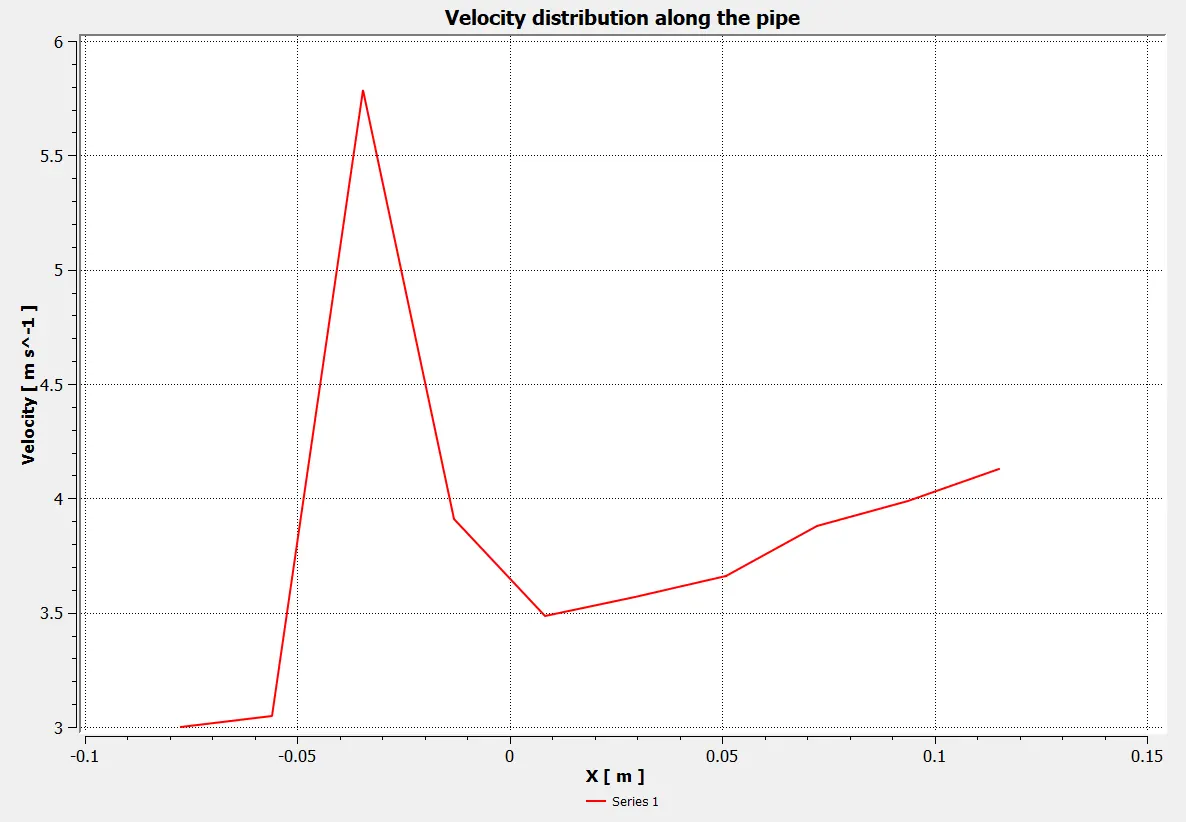
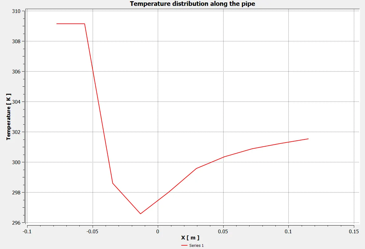
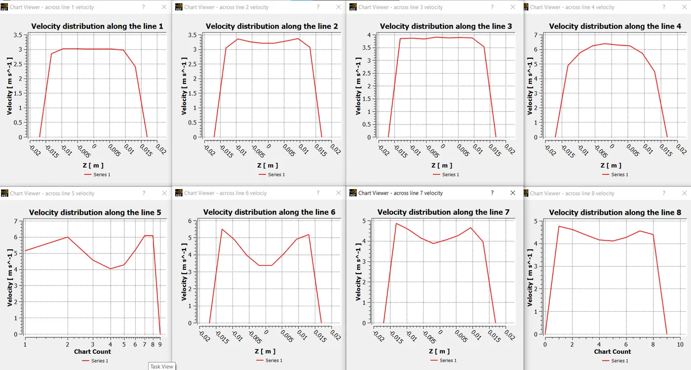
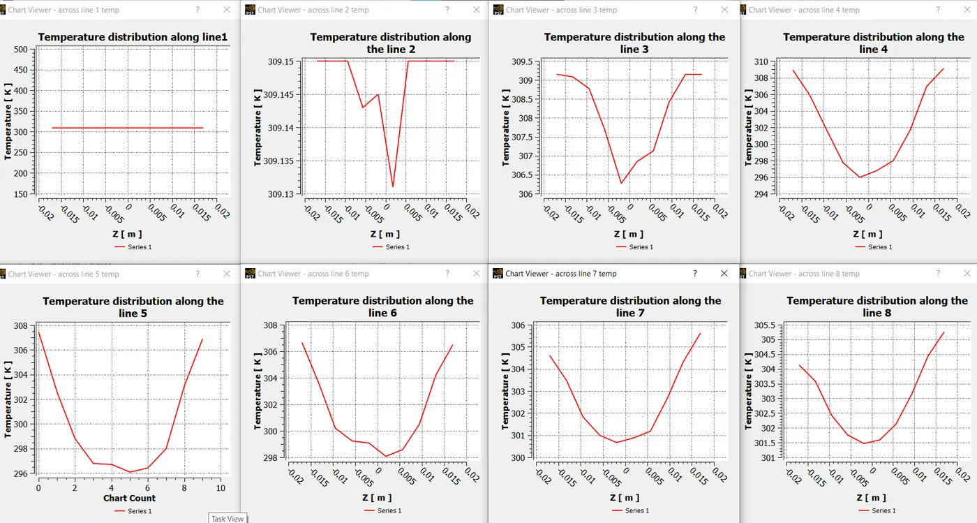
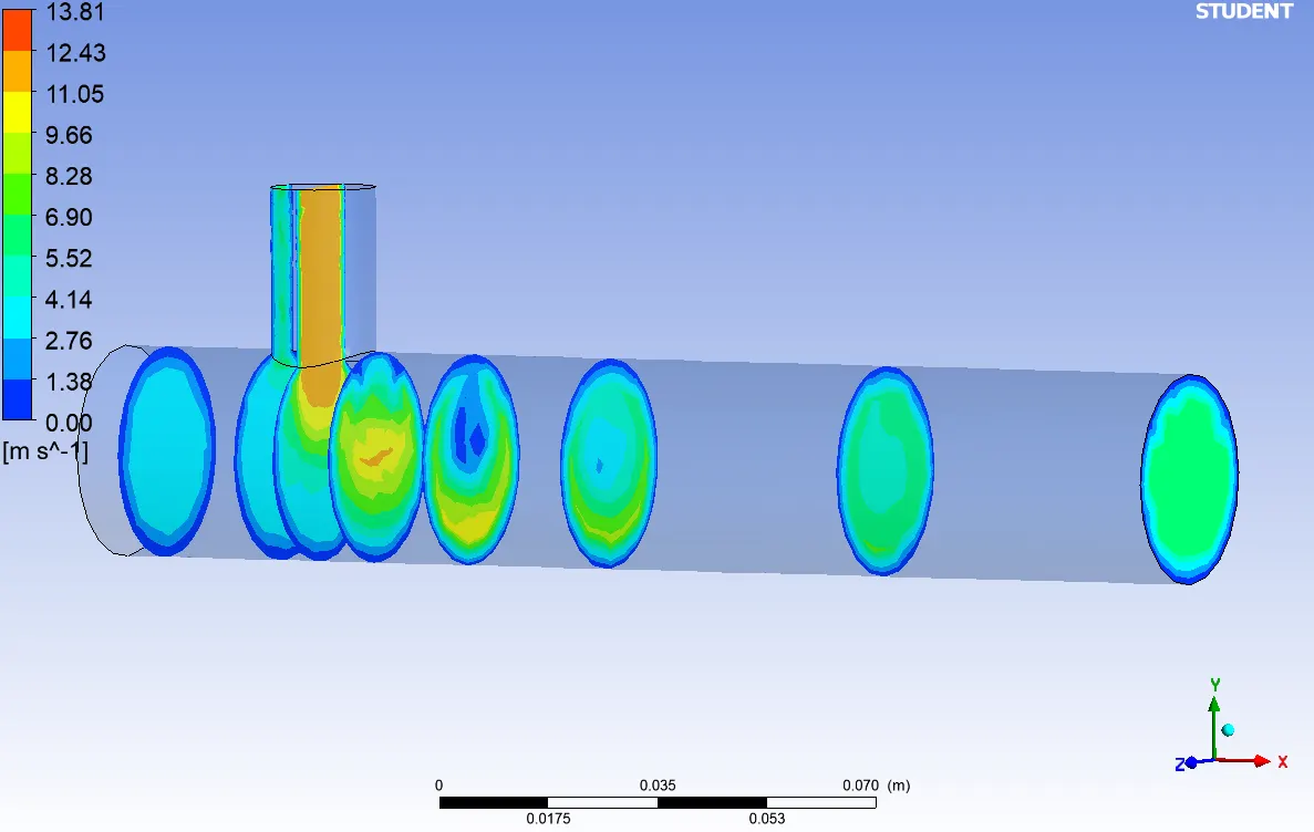
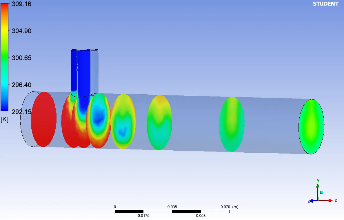
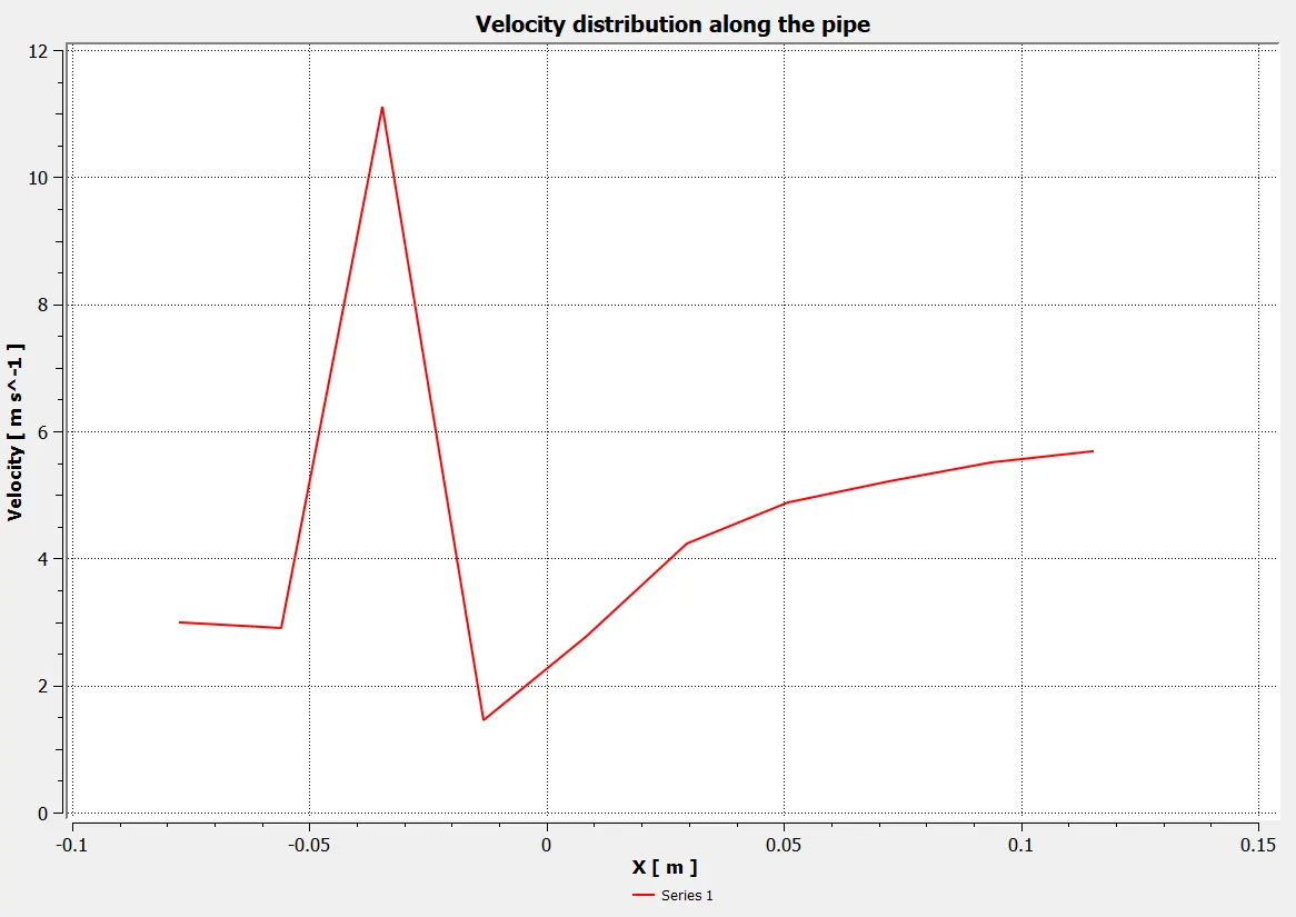
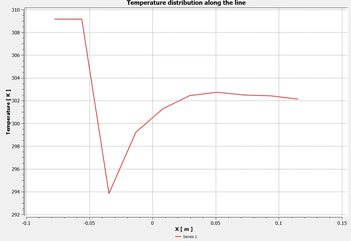
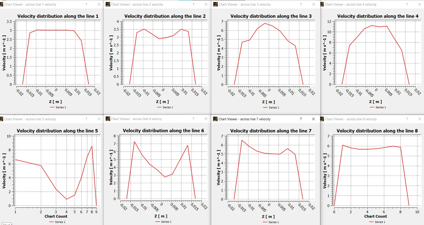
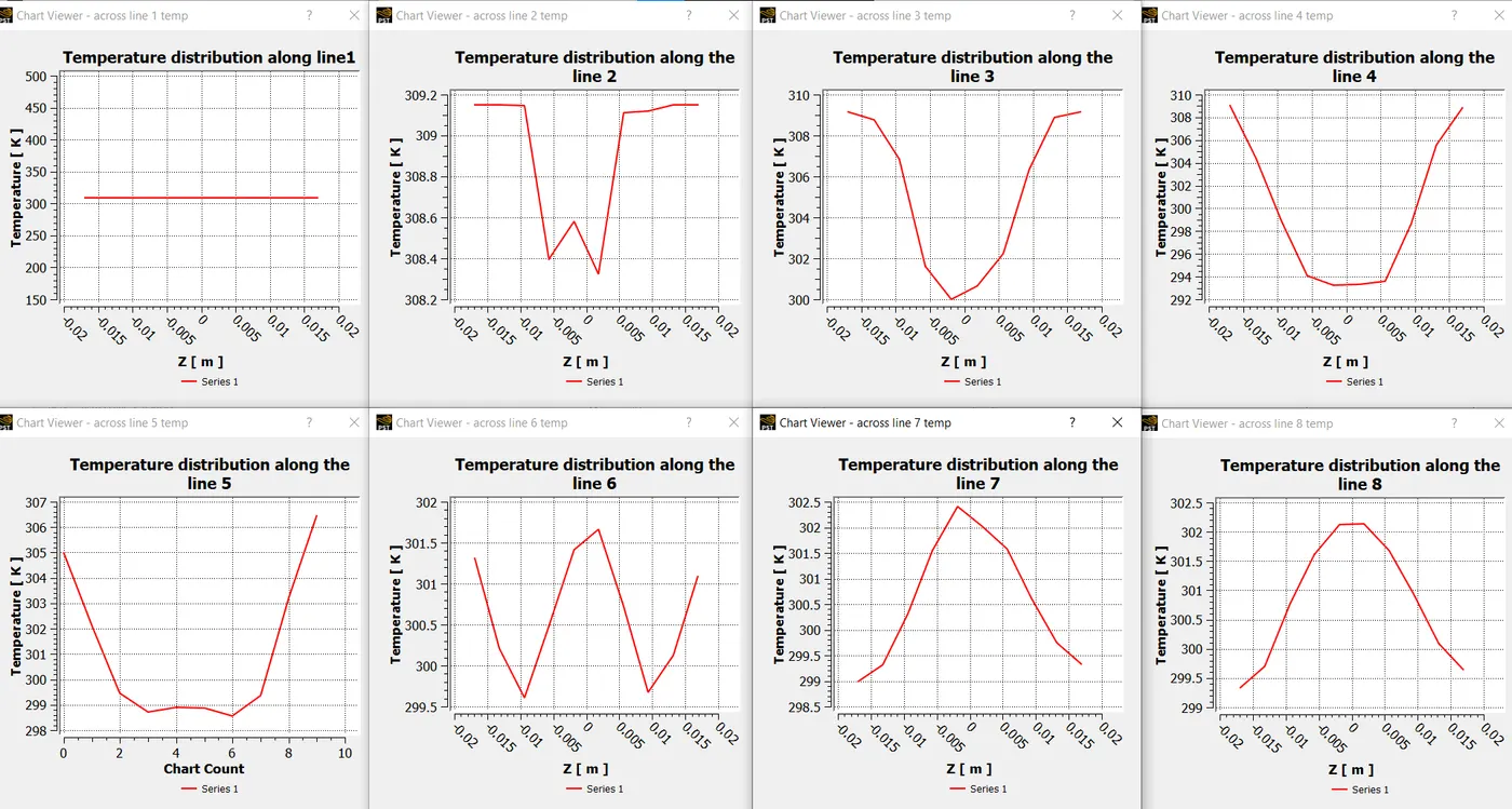
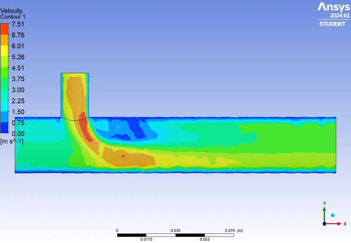
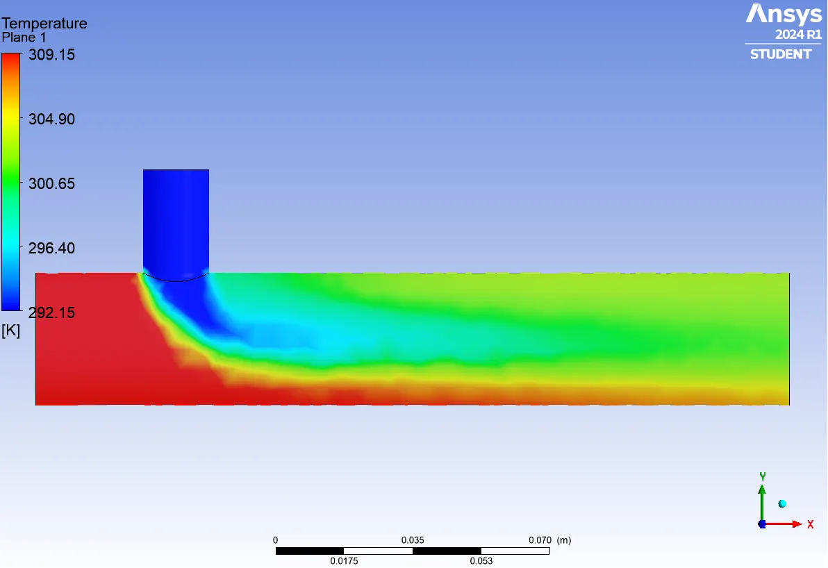
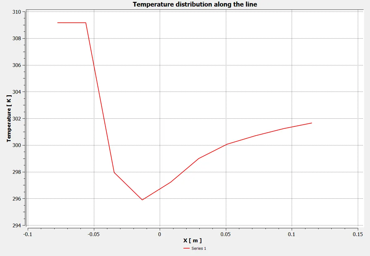
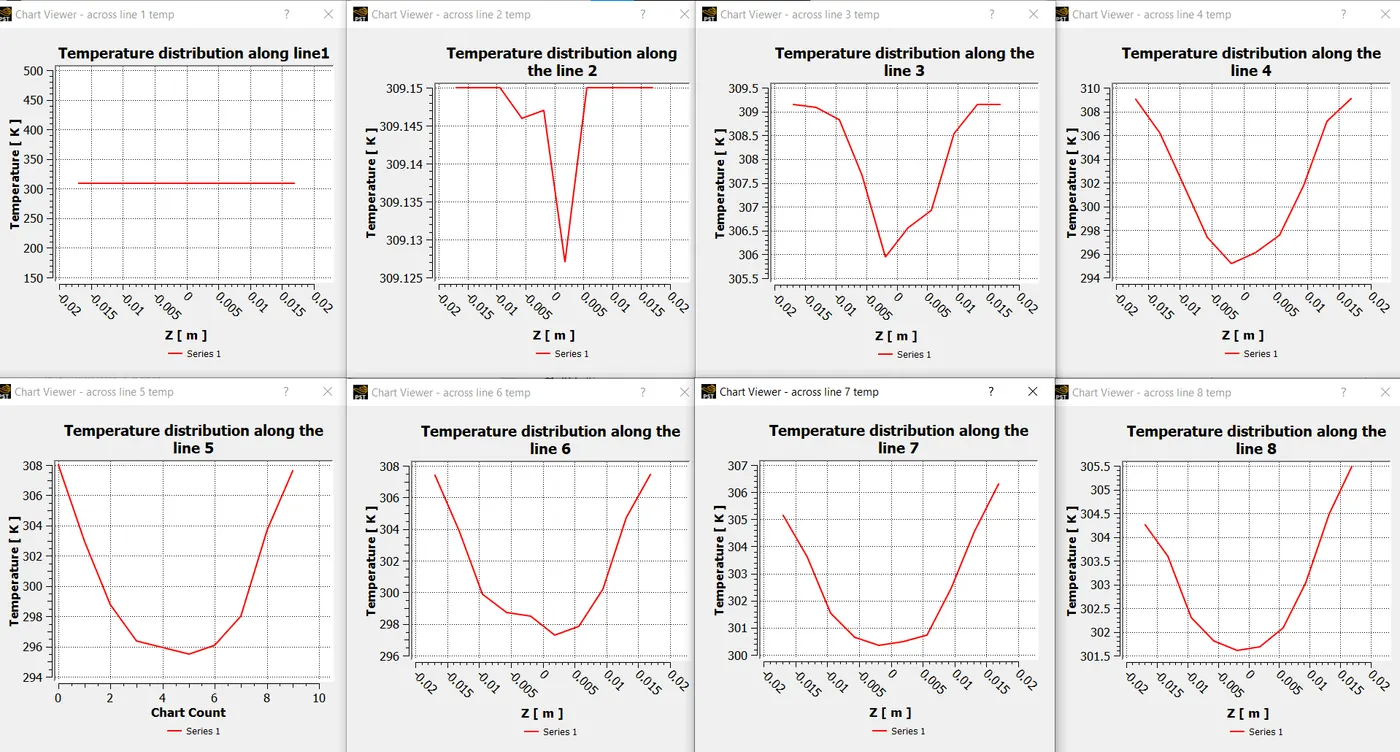
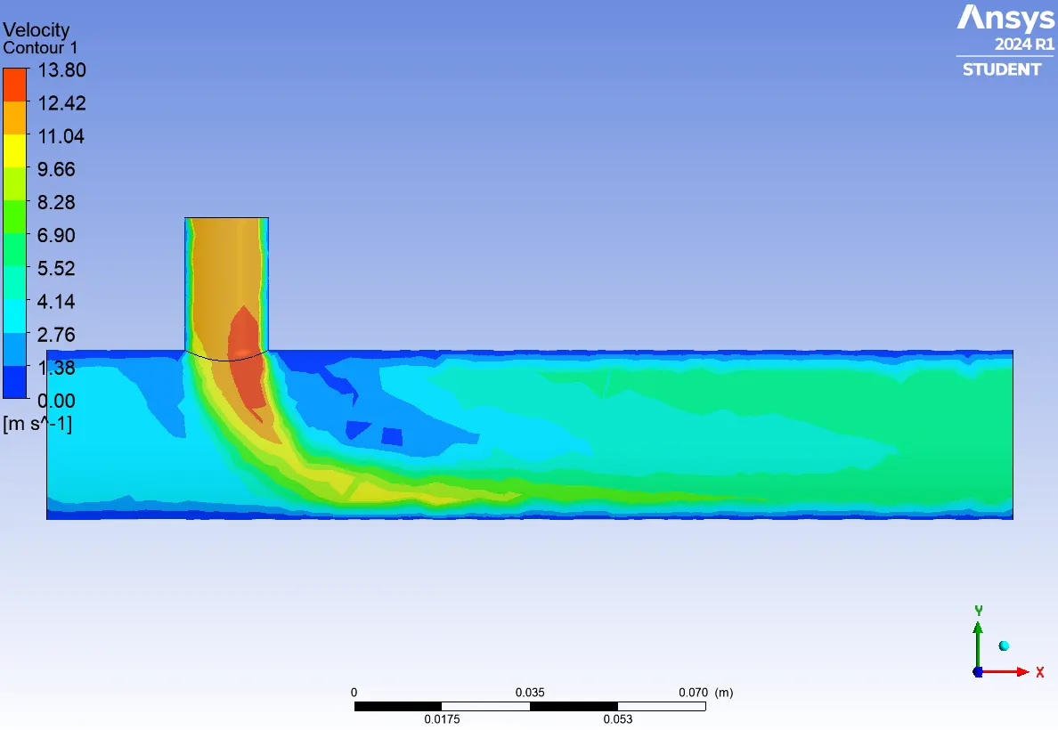
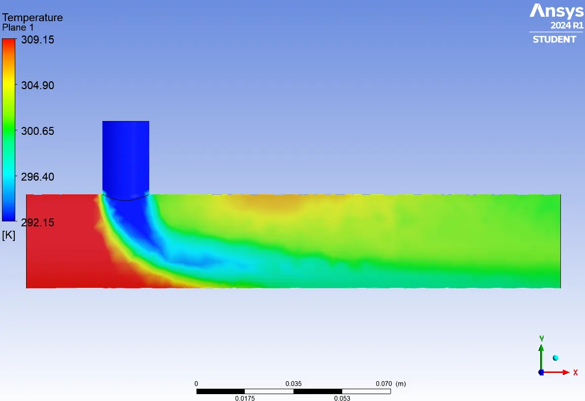
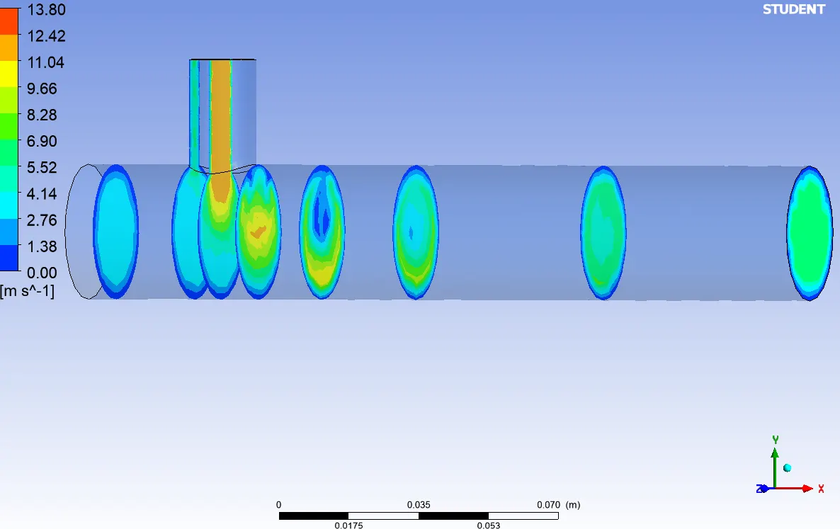
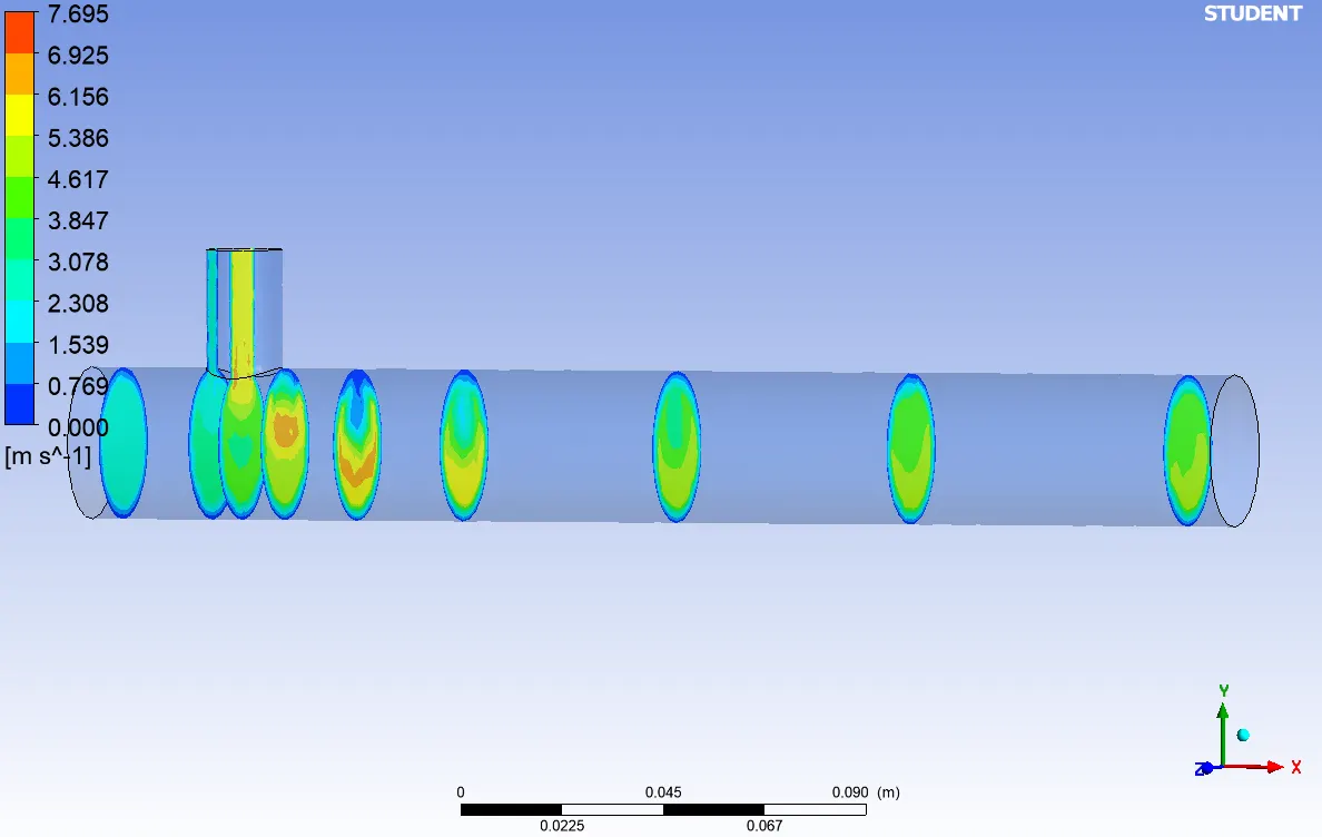
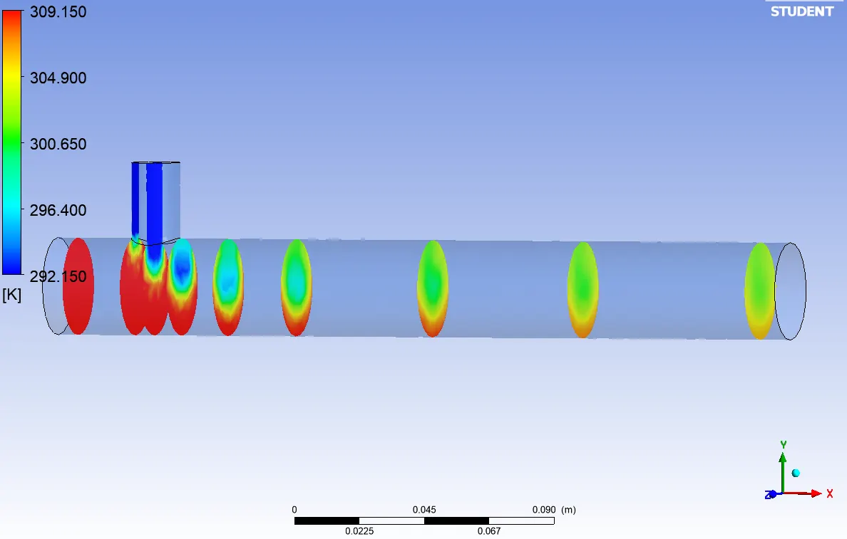
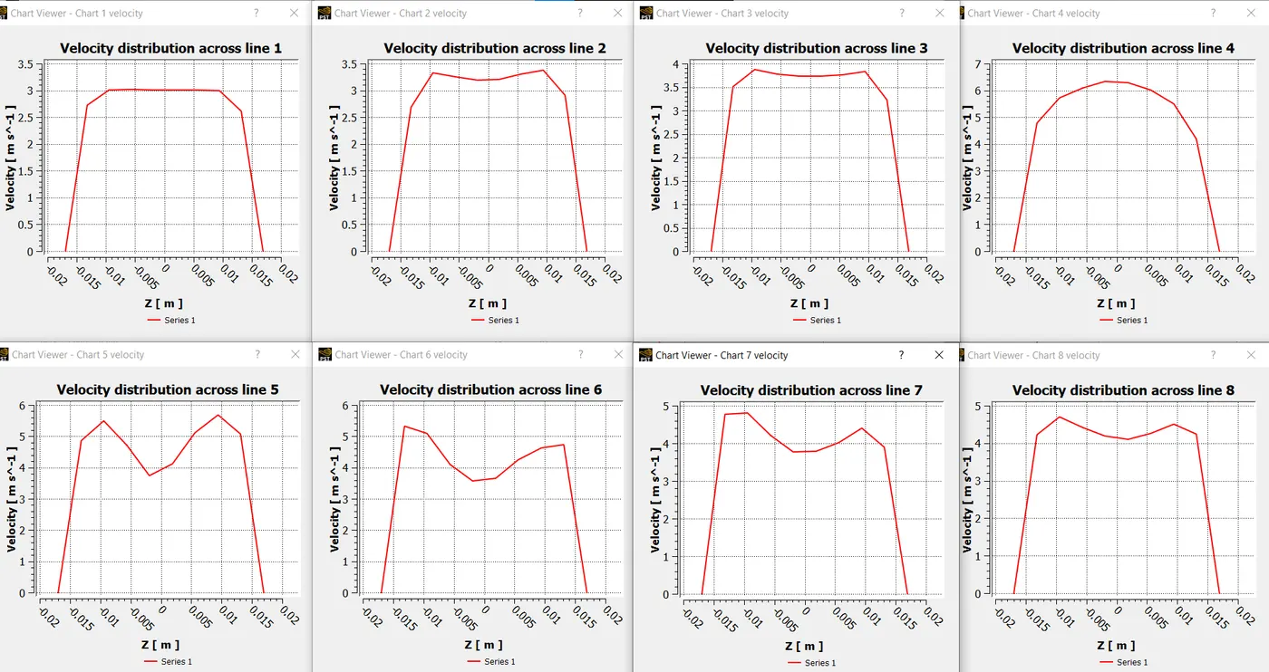
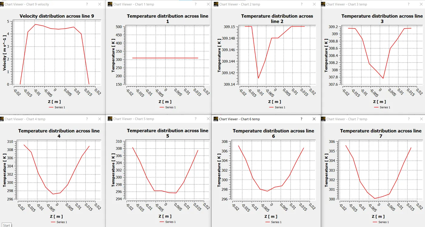
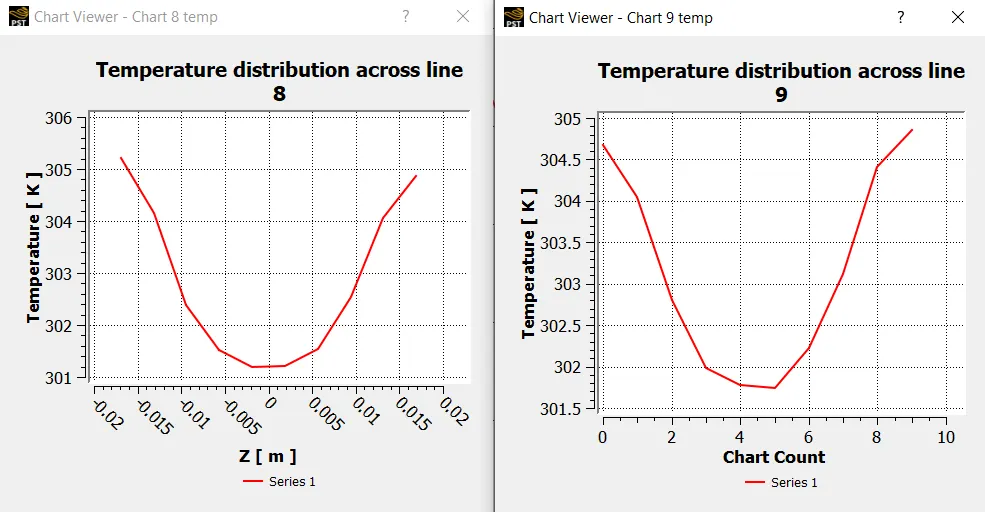
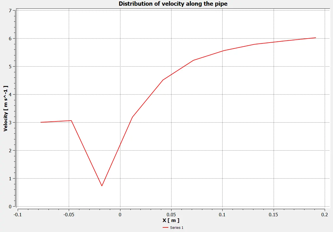
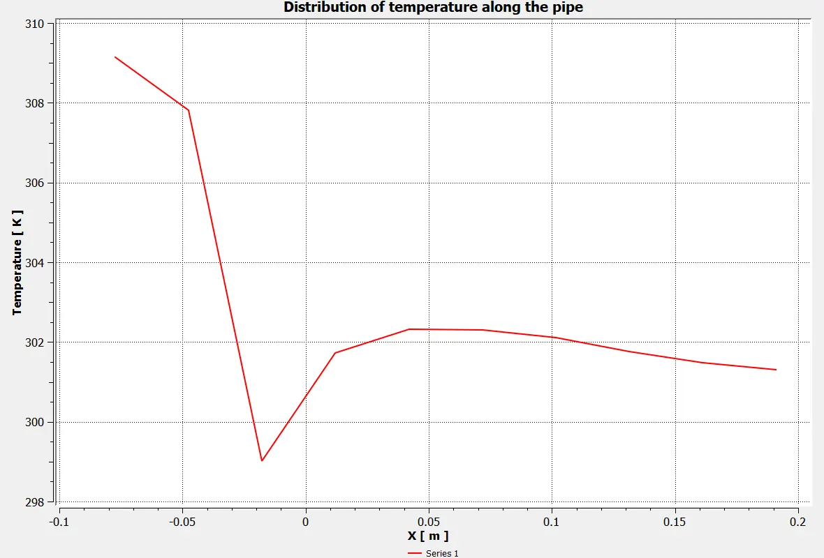
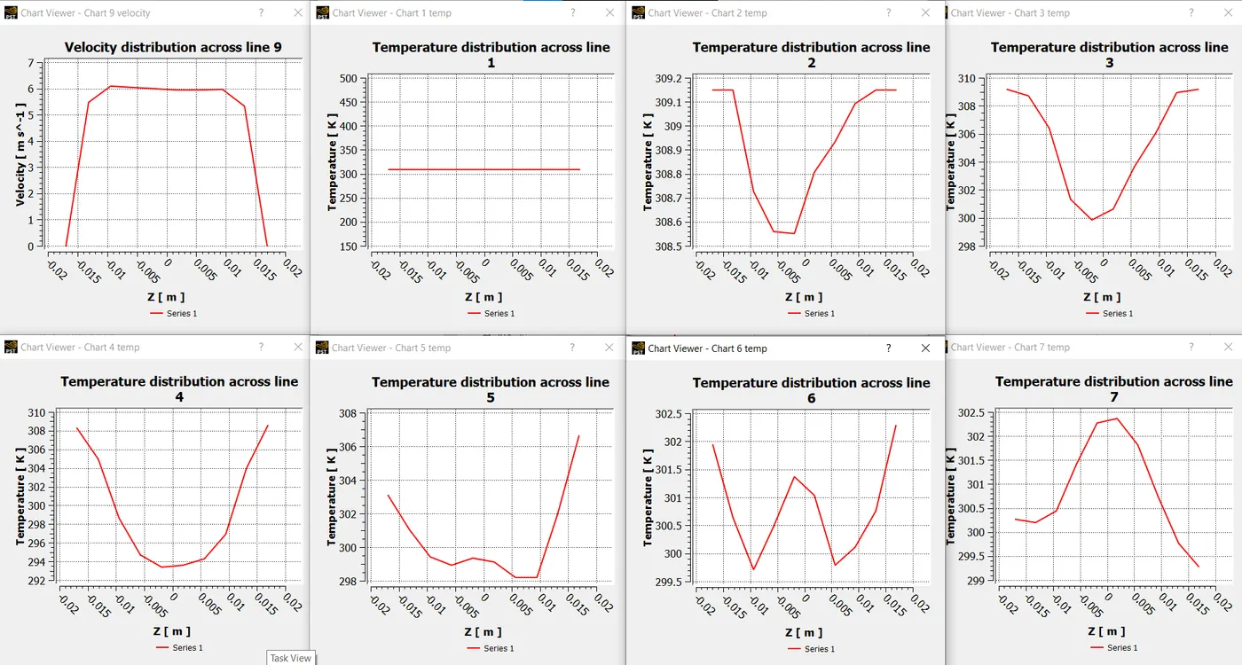
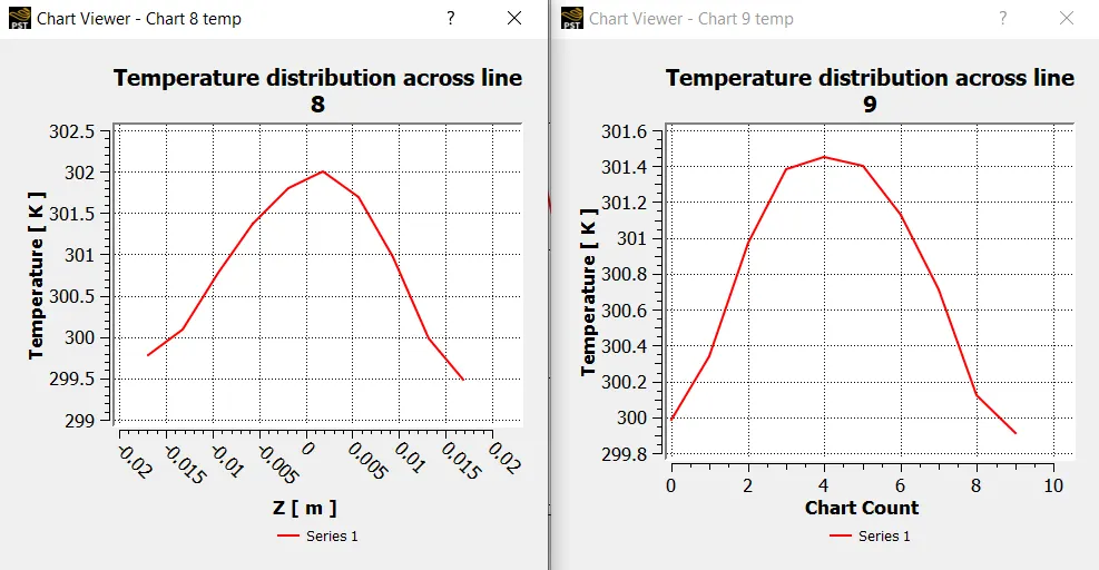
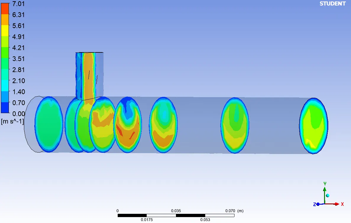
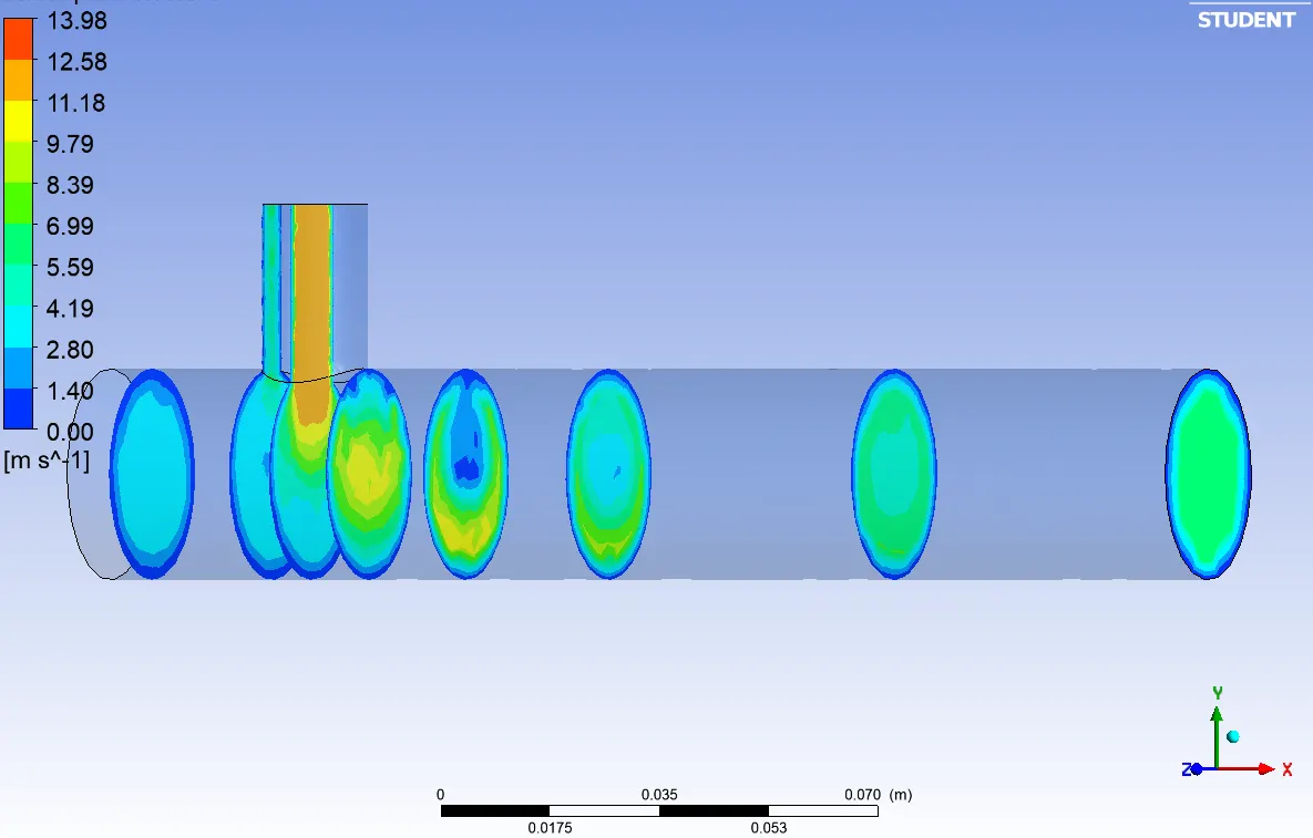
In CFD post, Render is used to alter the transparency of the extracted volume. Insert planes and set temperature and velocity as variables in the respective planes. Turn mesh lines on. Create contour plots. Create a line along the length and create a chart with the data source as the line created. Create a line along and across the length of the pipe. Create planes also in the same way. This process is repeated for the k omega model for short TEE and the best model is used in long Tee geometry. The planes across the length of the pipe are made at 8 different X values, -0.07, -0.049, -0.042, -0.032, -0.015, 0.01, 0.06, 0.115 numbered 1 to 8. A line is also made in these positions across the length of the pipe for getting line plots of velocity and temperature.
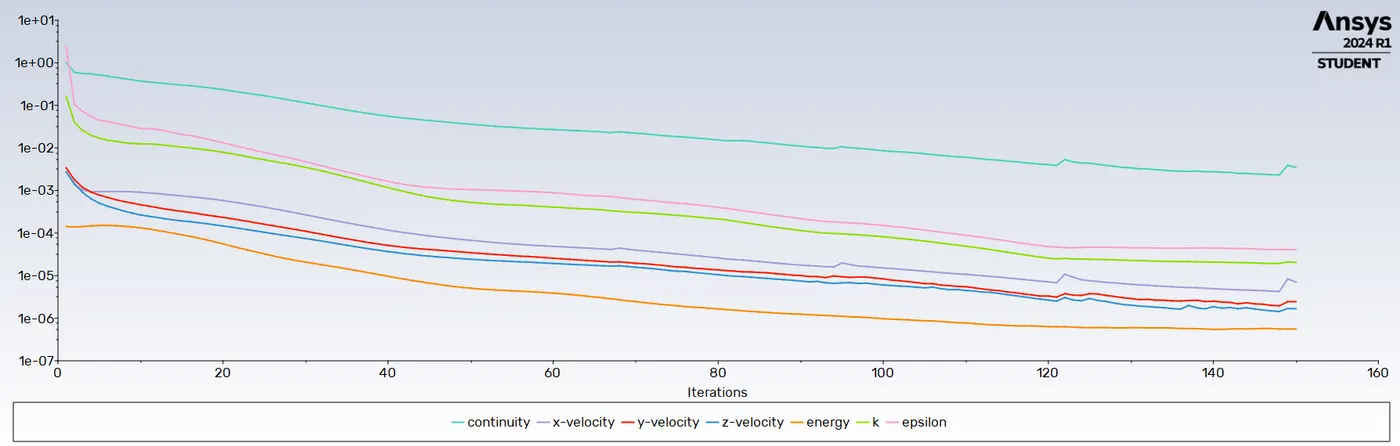
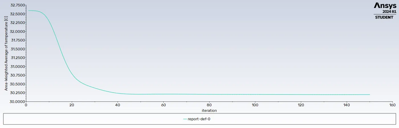
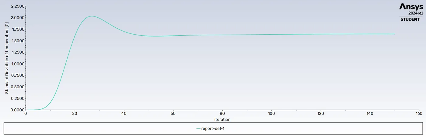
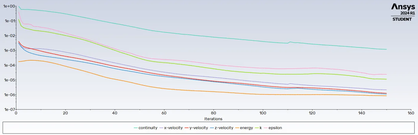
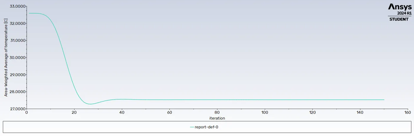
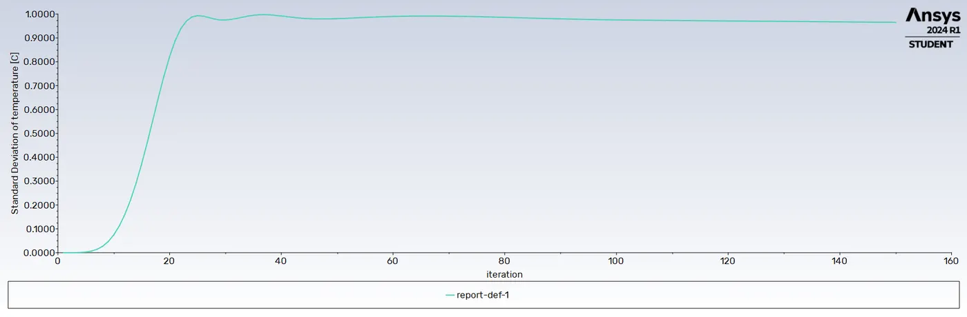
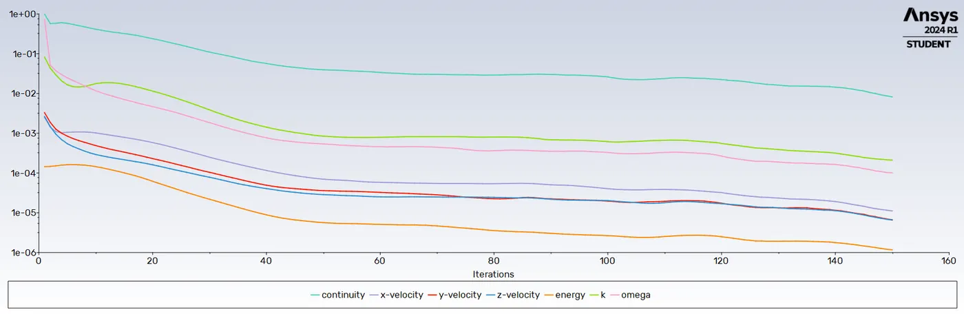
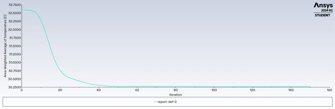
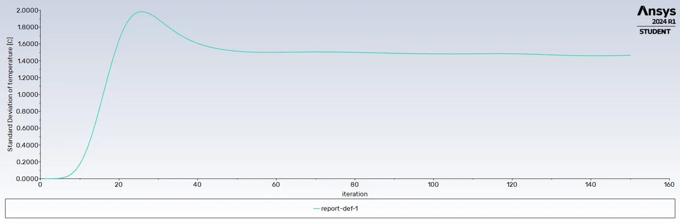
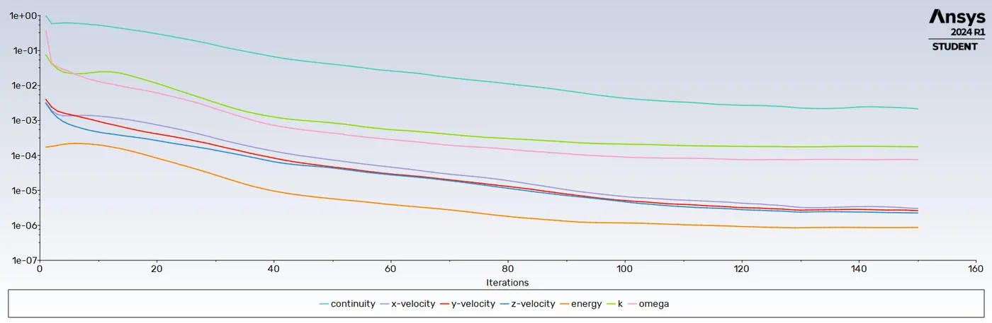
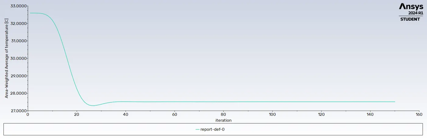
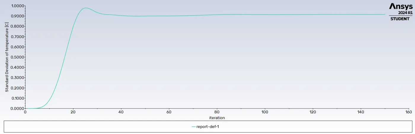
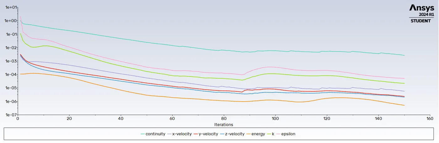
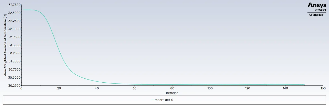
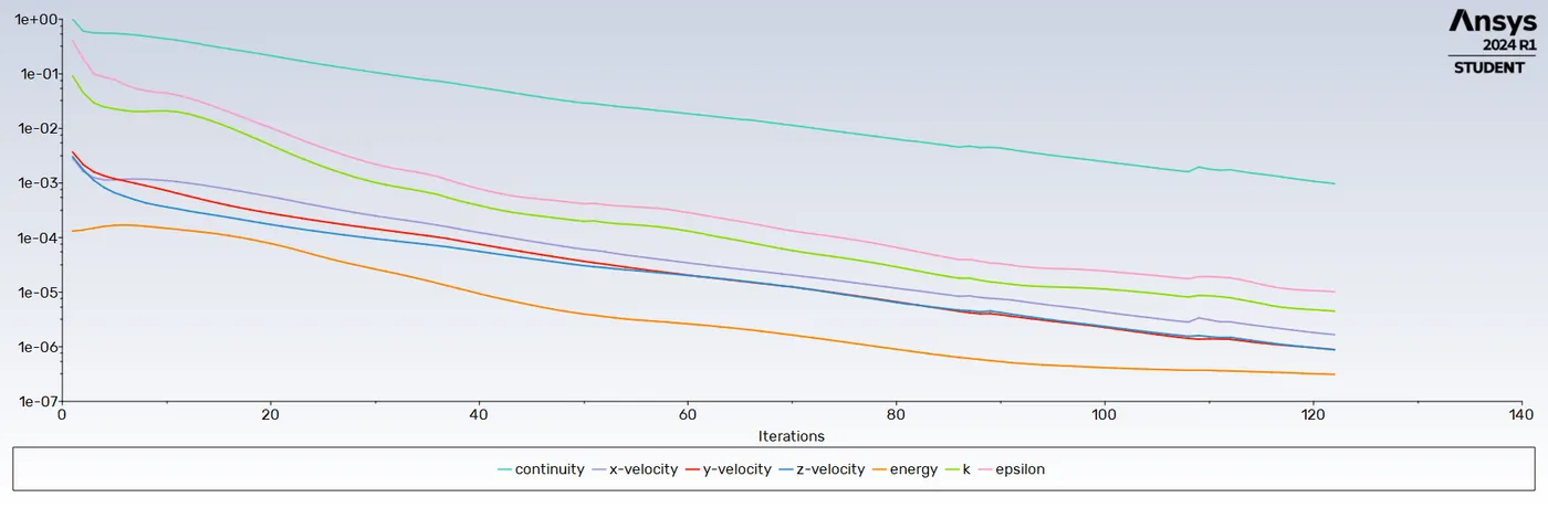
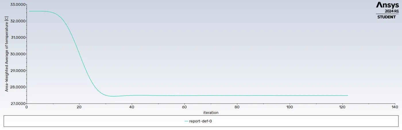
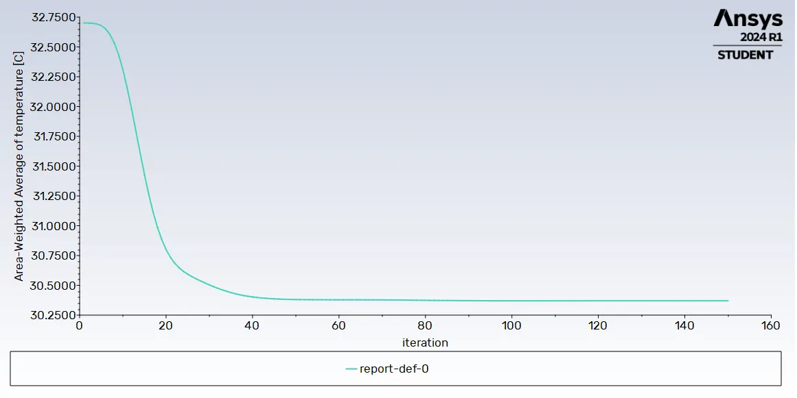
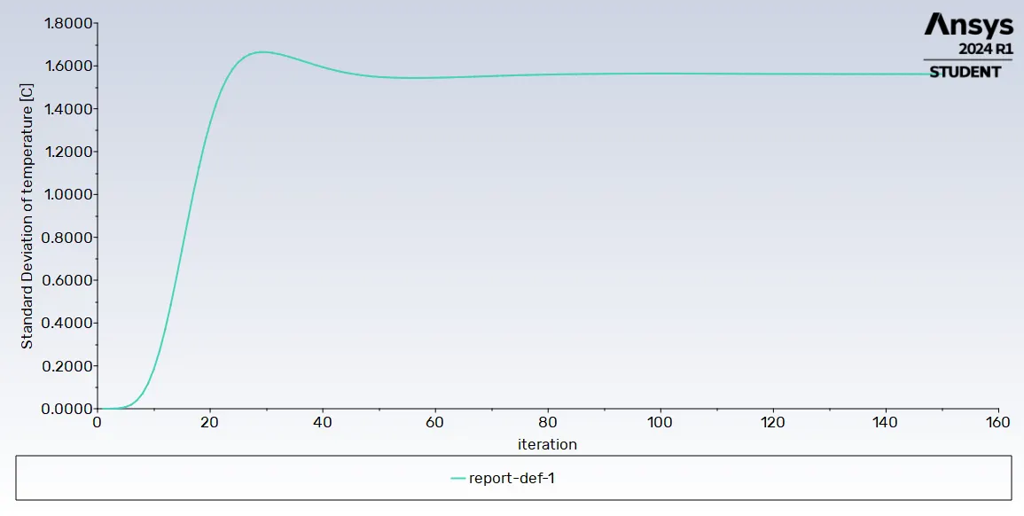
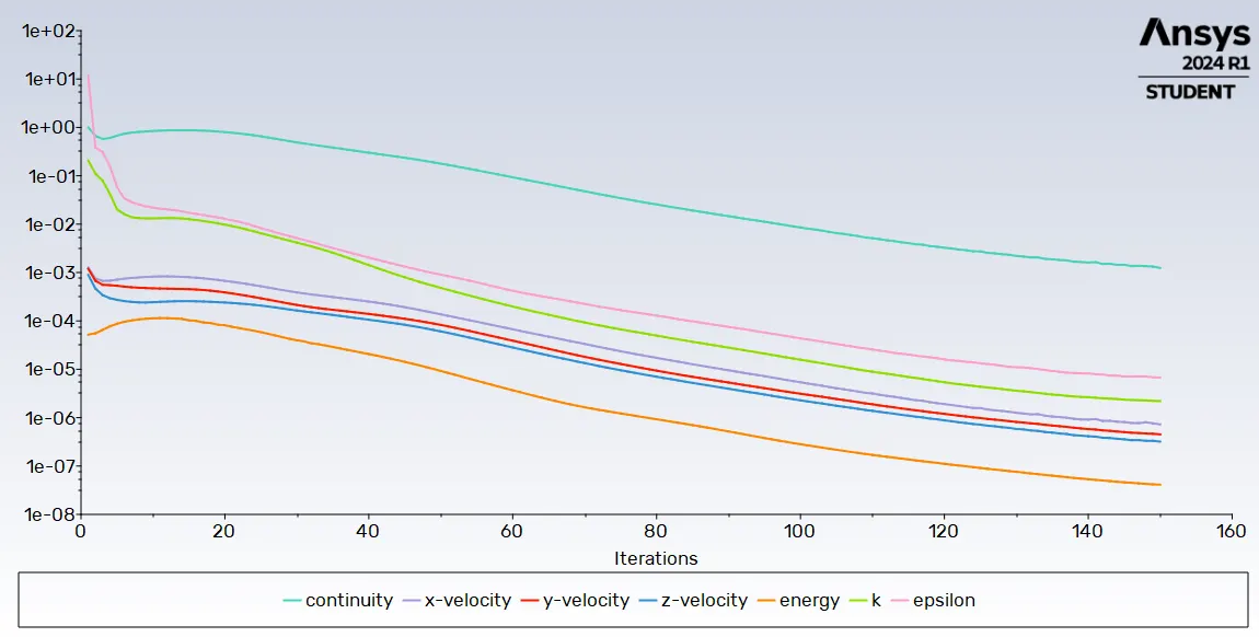
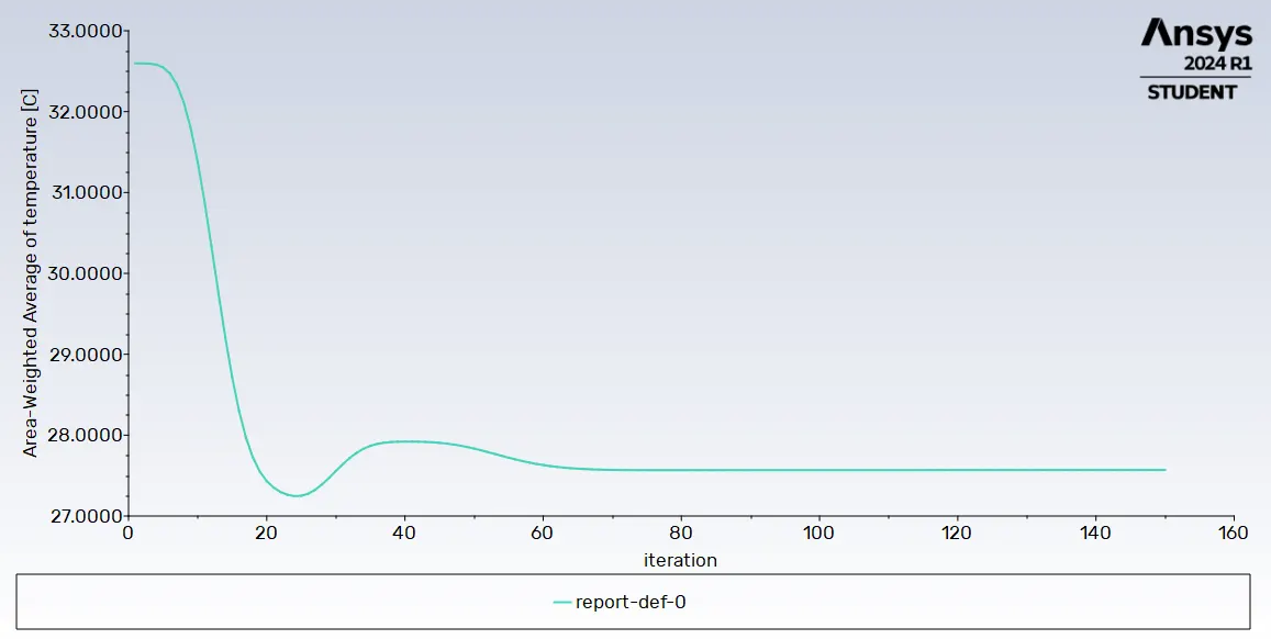
By comparing the scaled residue and standard deviation for each k epsilon and k omega model, k epsilon is better. k epsilon provides better uniform outlet temperature and velocity. It has both low scaled residue and area weighted average of outlet temperature. The scaled residue is less than 1e-06 for the last iteration, and the area-weighted average of outlet temperature is less than 30.25 0C (for momentum ratio 2).
Average temperature
Number of iterations
| case 1, k epsilon | case 1, k epsilon | case 1, k omega | case 1, k omega | case 2, k epsilon | case 2, k epsilon | |
|---|---|---|---|---|---|---|
| momentum ratio2 | momentum ratio4 | momentum ratio2 | momentum ratio4 | momentum ratio2 | momentum ratio4 | |
| cell count | 12732 | 12732 | 12732 | 12732 | 15731 | 15732 |
| Avg. outlet temperature | 30.24 0C | 27.5 0C | 30.25 0C | 27.5 0C | 30.25 0C | 27.5 0C |
| no. of iterations for convergence | 50 | 40 | 50 | 40 | 60 | 40 |
Case:1
Geometry:
Extract volume
Mesh:
Generated Mesh
Section Plane
Mesh metric Element Quality
k epsilon, momentum ratio 2:
Set up:
Scaled residuals
Weighted Average
Standard deviation
CFD Post:
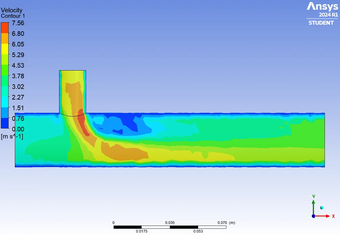
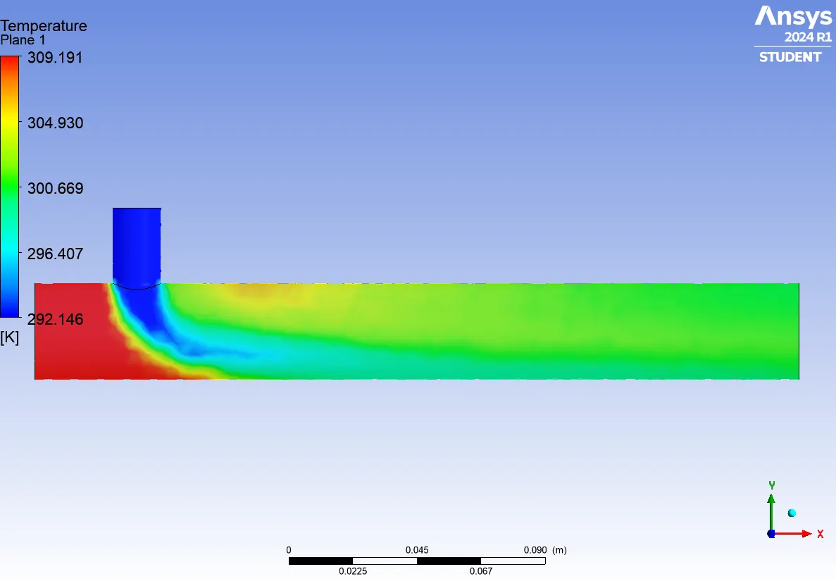
Velocity temperature contour plots:
Along the pipe:
Across the pipe:
Velocity:
Temperature:
Velocity temperature line plots:
Along the pipe:
Across the pipe:
k epsilon, momentum ratio 4:
Set up:
Scaled residuals:
Area weighted average outlet temperature:
Standard deviation of outlet temperature:
CFD Post:
Velocity and temperature contour plots:
Along the pipe:
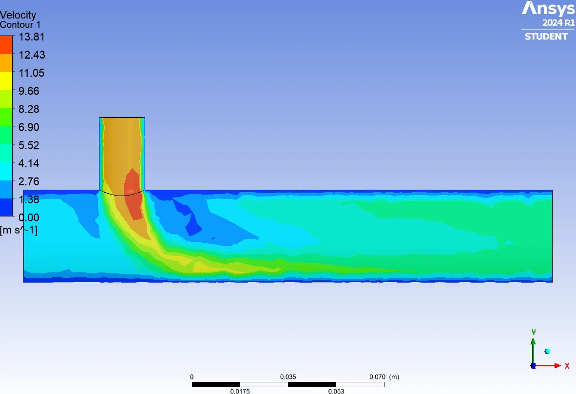
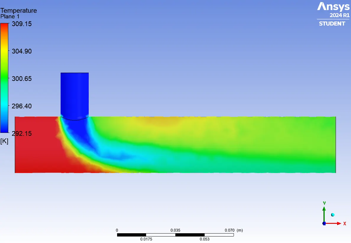
Across the pipe:
Velocity:
Temperature:
Velocity and temperature line plots:
Along the pipe:
Across the pipe:
k omega, momentum ratio 2:
Set up:
Scaled residuals
Weighted average
Standard deviation
CFD Post:
Velocity and temperature contour plots:
Along the pipe:
Across the pipe:
Velocity: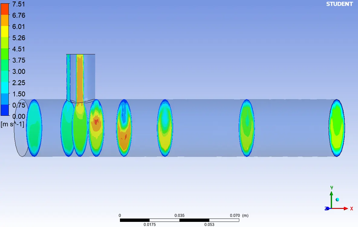
Temperature: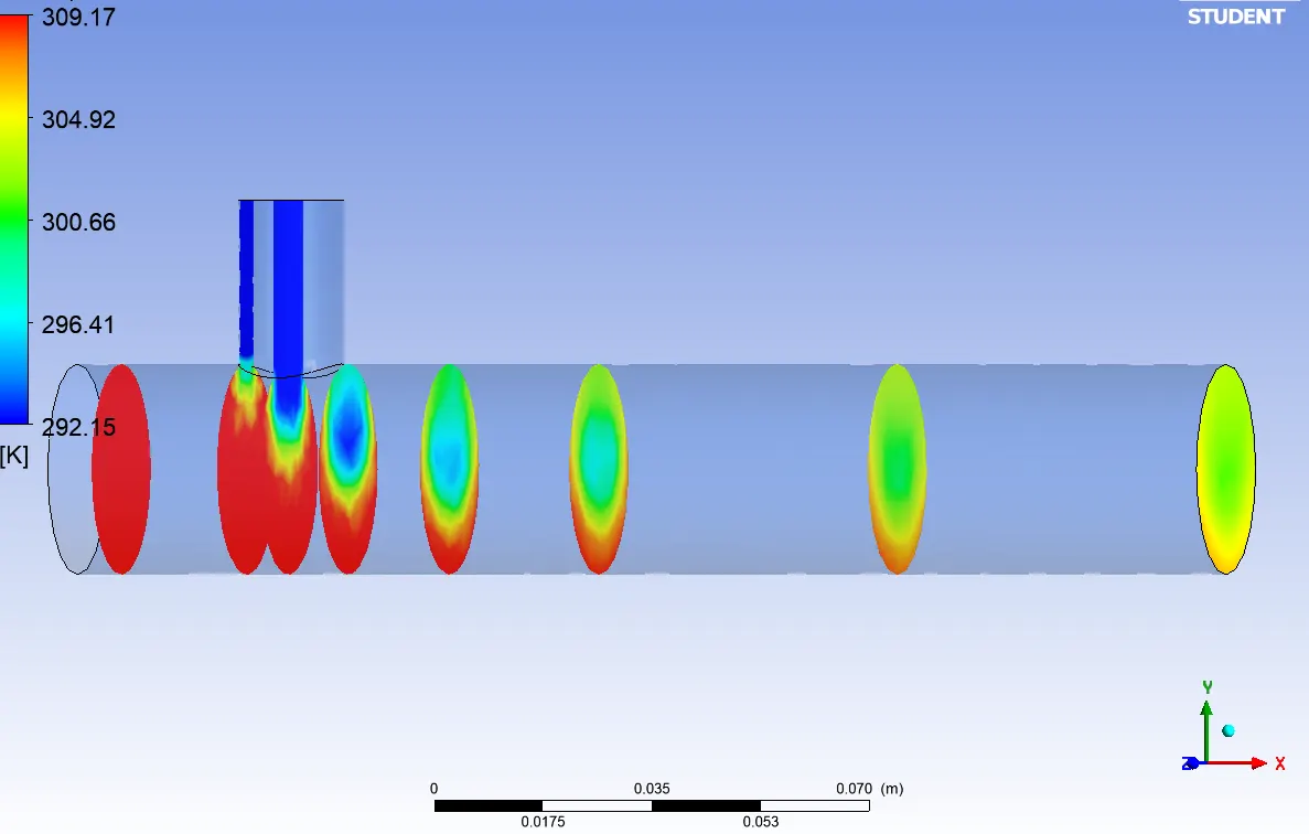
Temperature and velocity line plot:
Along the pipe: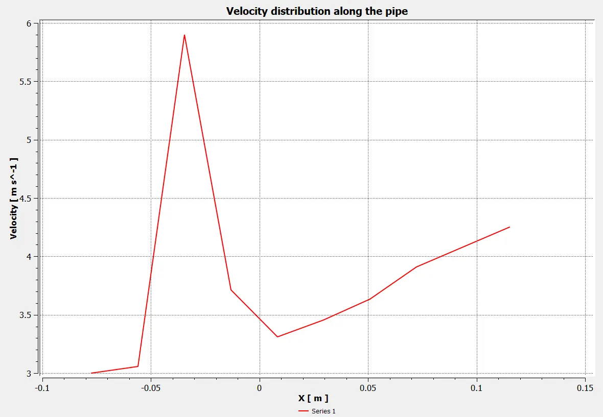
Across the pipe:
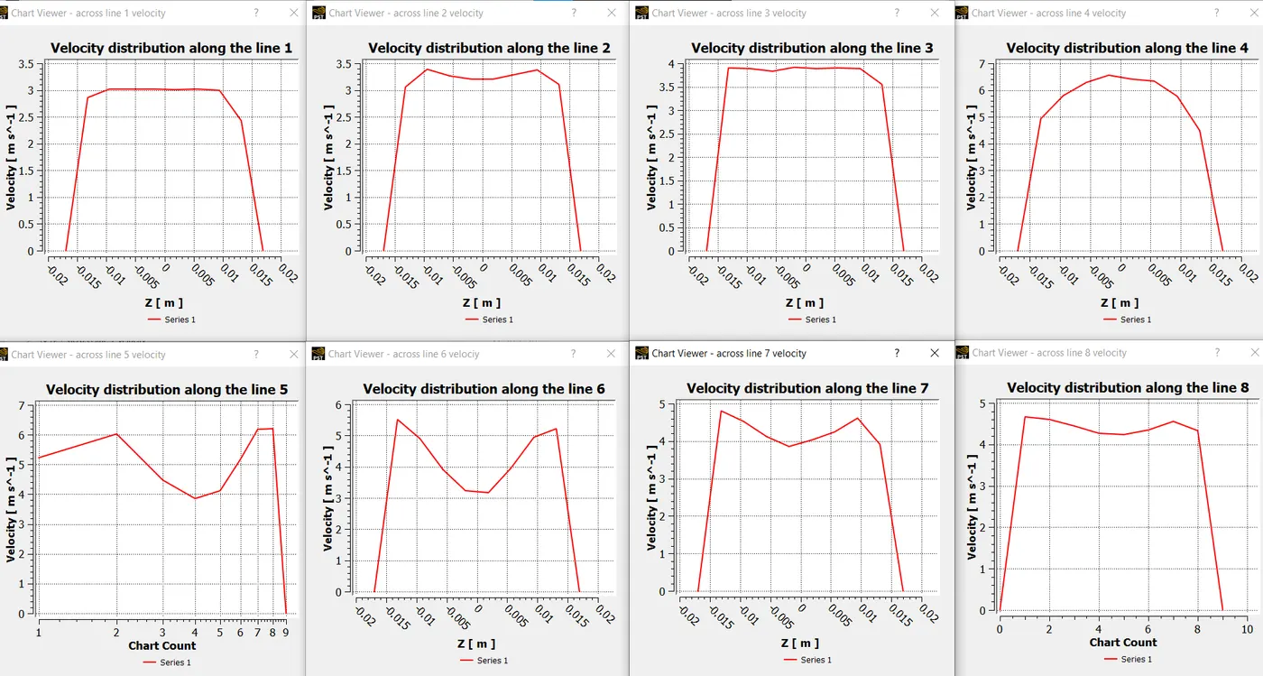
k omega, momentum ratio 4:
Set up:
Scaled residuals
Area weighted average of outlet temperature
Standard deviation of outlet temperature
Set up:
Velocity and temperature contour:
Along the pipe:
Across the pipe:
Velocity:
Temperature: 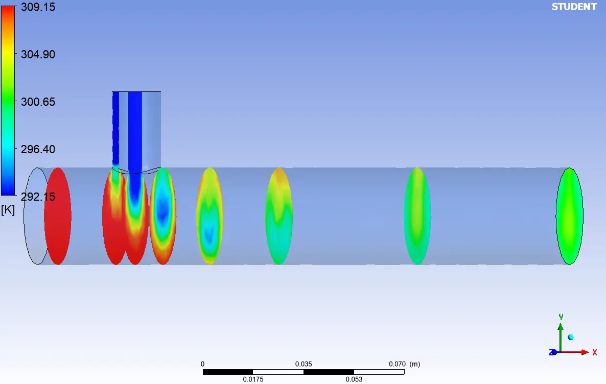
Velocity and temperature line plot:
Along the pipe:
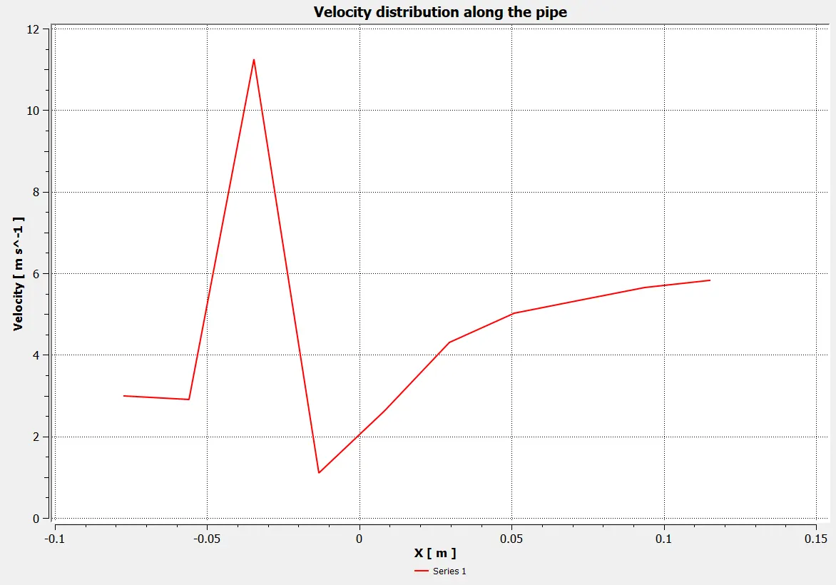
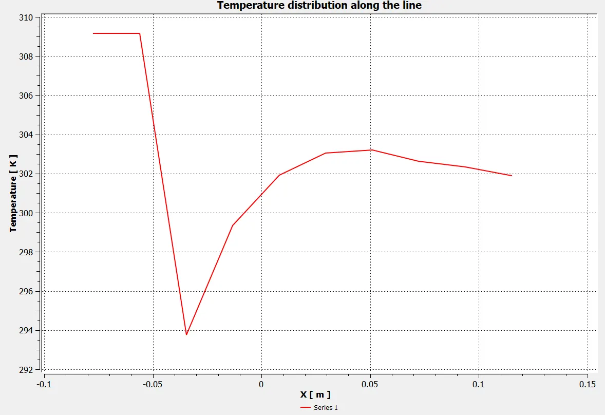
Across the pipe:
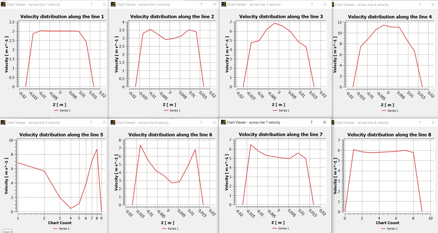
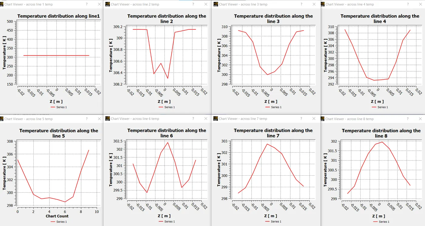
Case:2
Geometry:
Extract volume
Mesh:
Generated Mesh
Section Plane
Mesh metric element quality
Set up:
k epsilon, momentum ratio 2:
Scaled Residuals
Weighted average
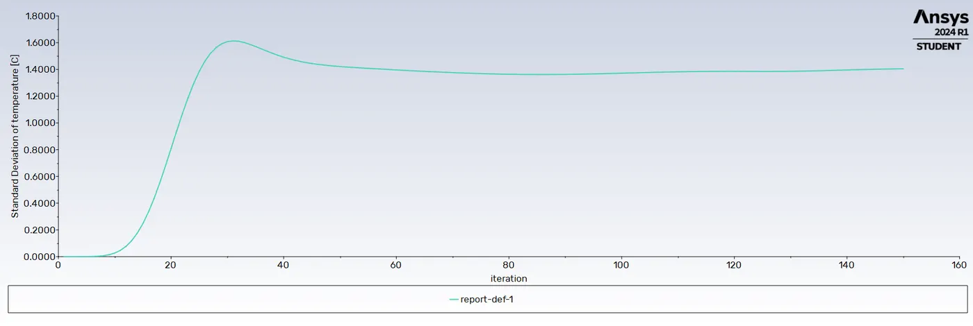
Standard deviation
CFD Post:
Velocity and temperature contour plots:
Along the pipe:
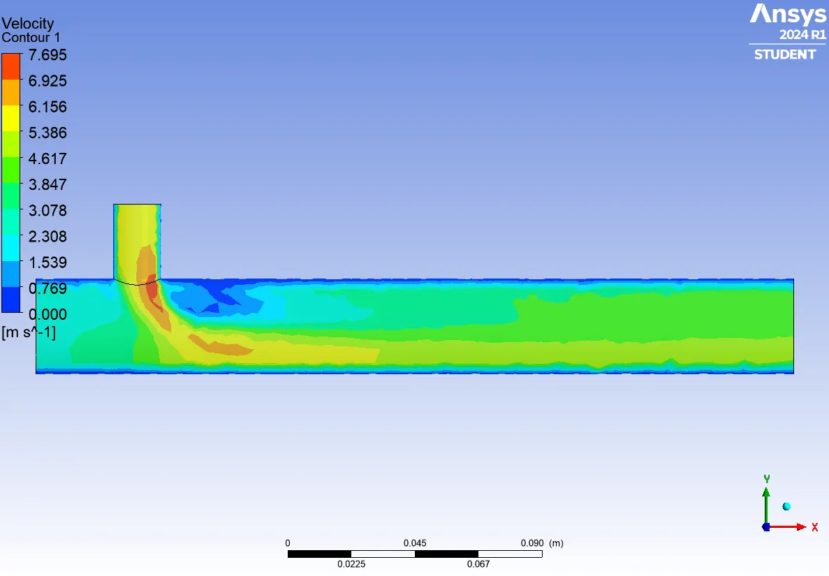
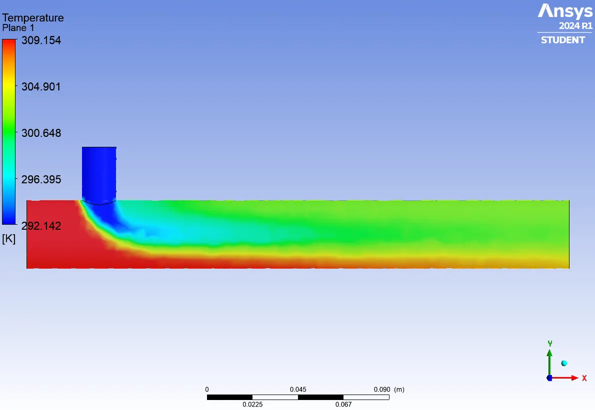
Across the pipe:
Velocity:
Temperature:
Velocity and temperature line plots:
Along the pipe:
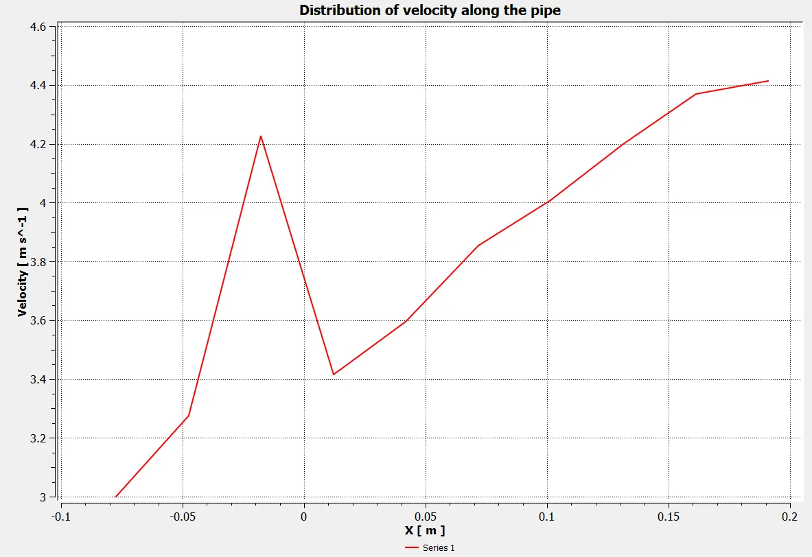
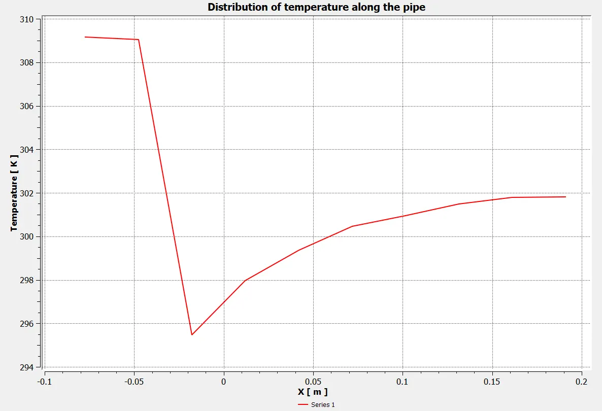
Across the pipe:
k epsilon, momentum ratio 4:
Set up:
Scaled residual
Area weighted average of outlet temperature
Standard deviation of outlet temperature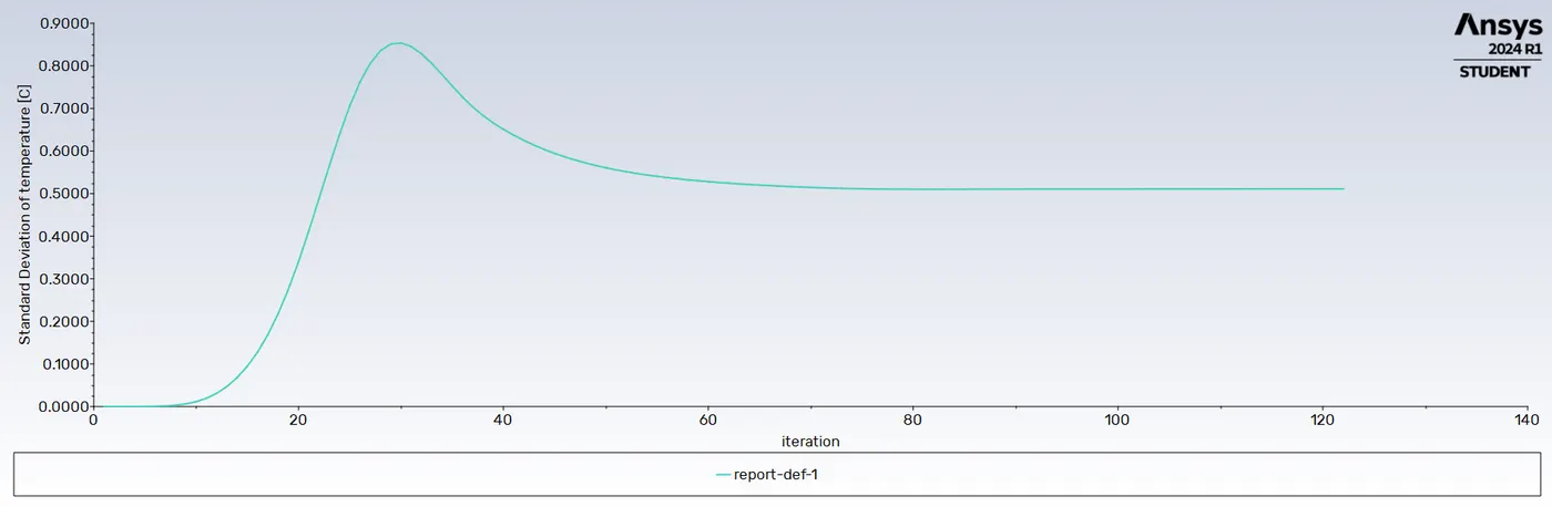
CFD Post:
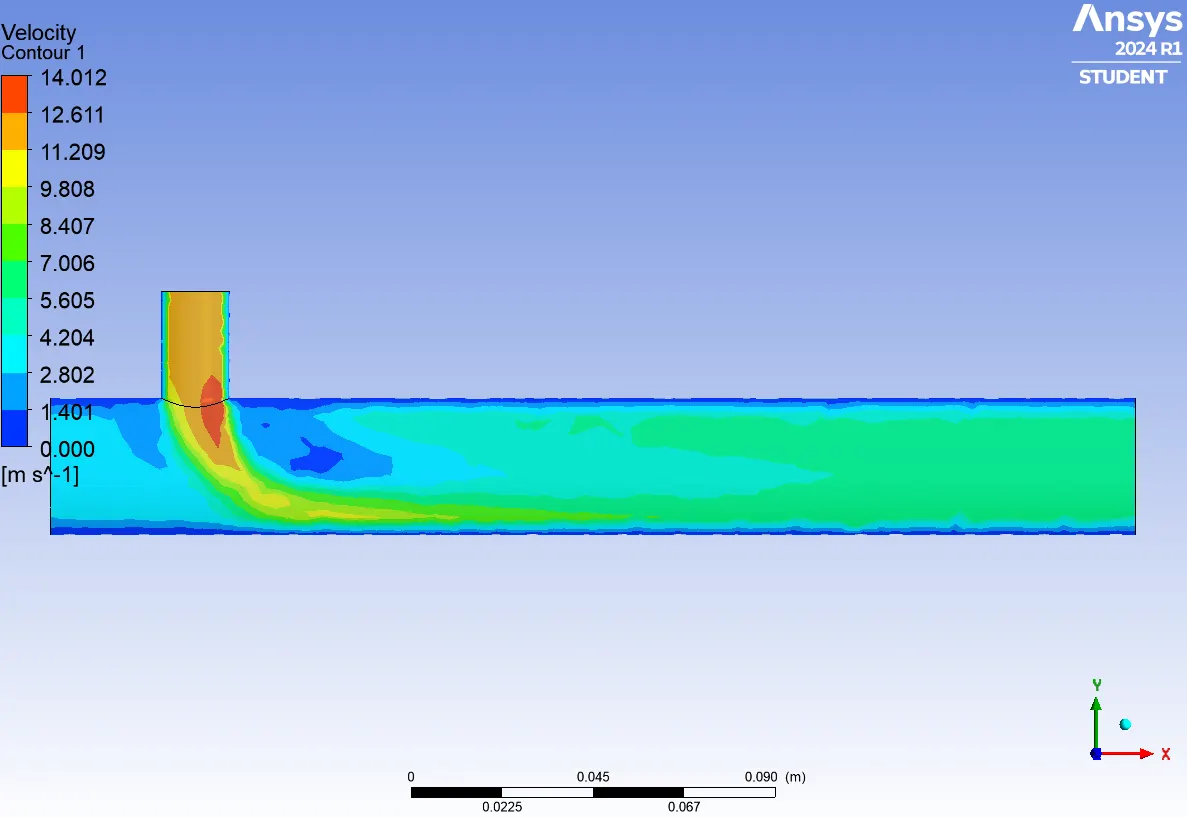
Velocity and temperature contour plot:
Along the pipe:
Across the pipe:
Velocity: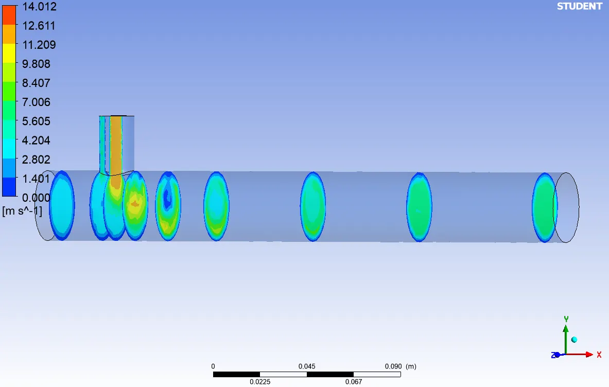
Temperature: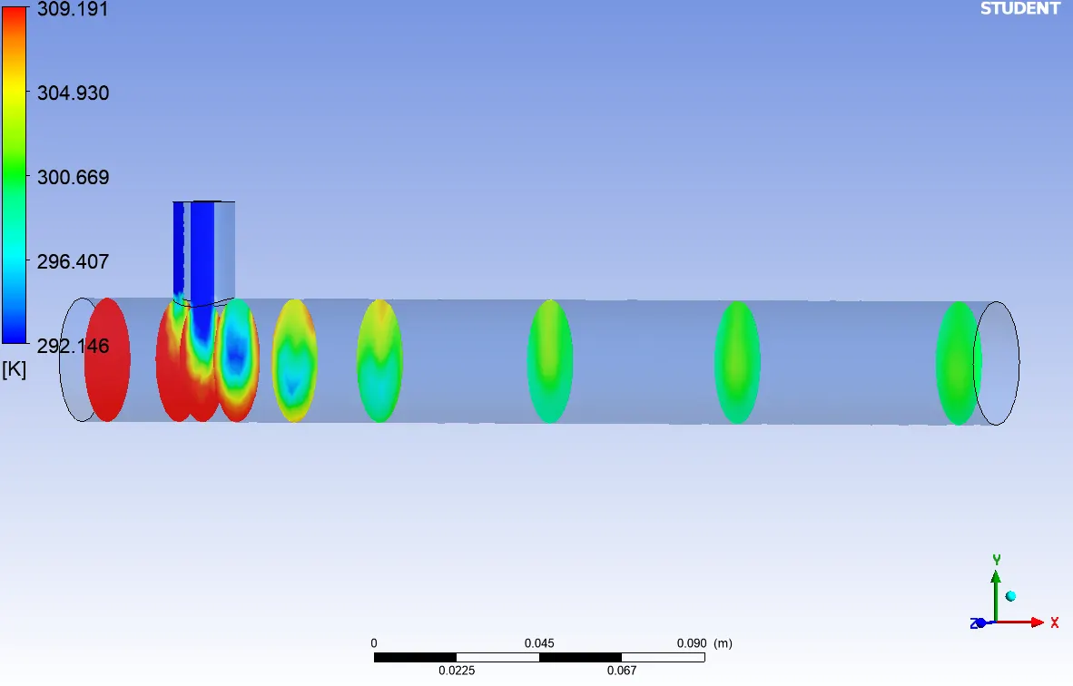
Velocity and temperature line plot:
Along the pipe
Across the pipe: 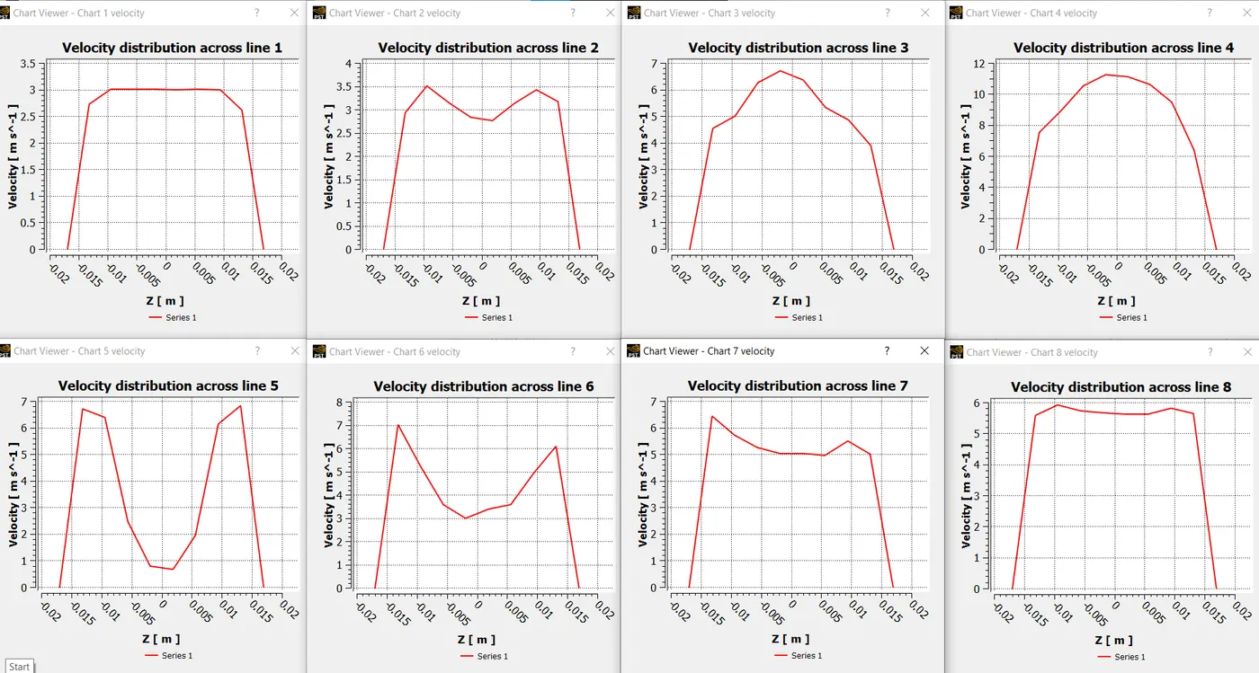
Mesh independent study:
case 1:
k epsilon, momentum ratio 2:
Mesh length 0.005 m:
 Set up:
Scaled residuals 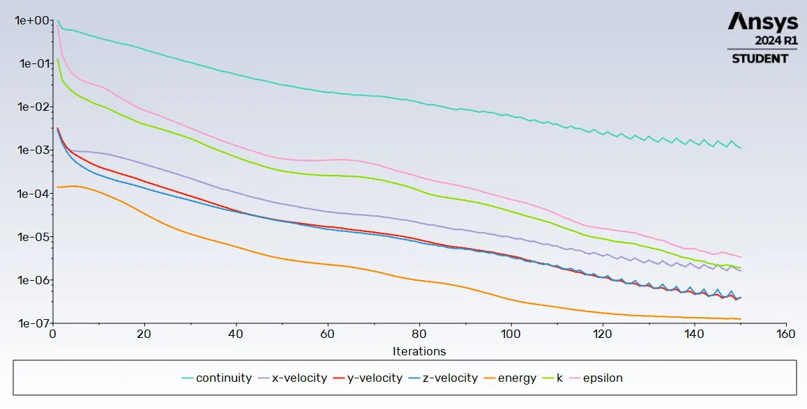 Area weighted average of outlet temperature
  Standard deviation
  CFD Post: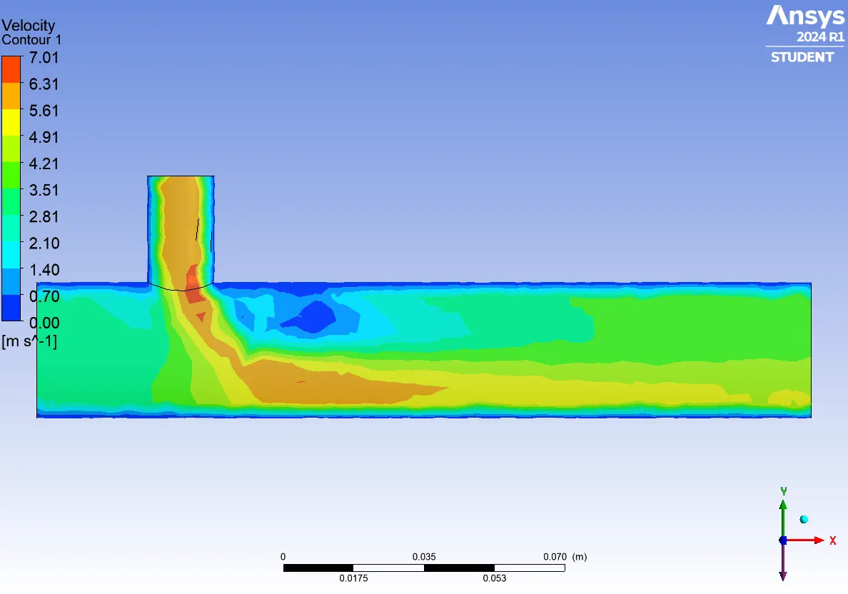
 Velocity:
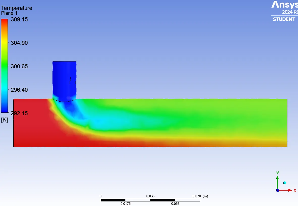
  Temperature: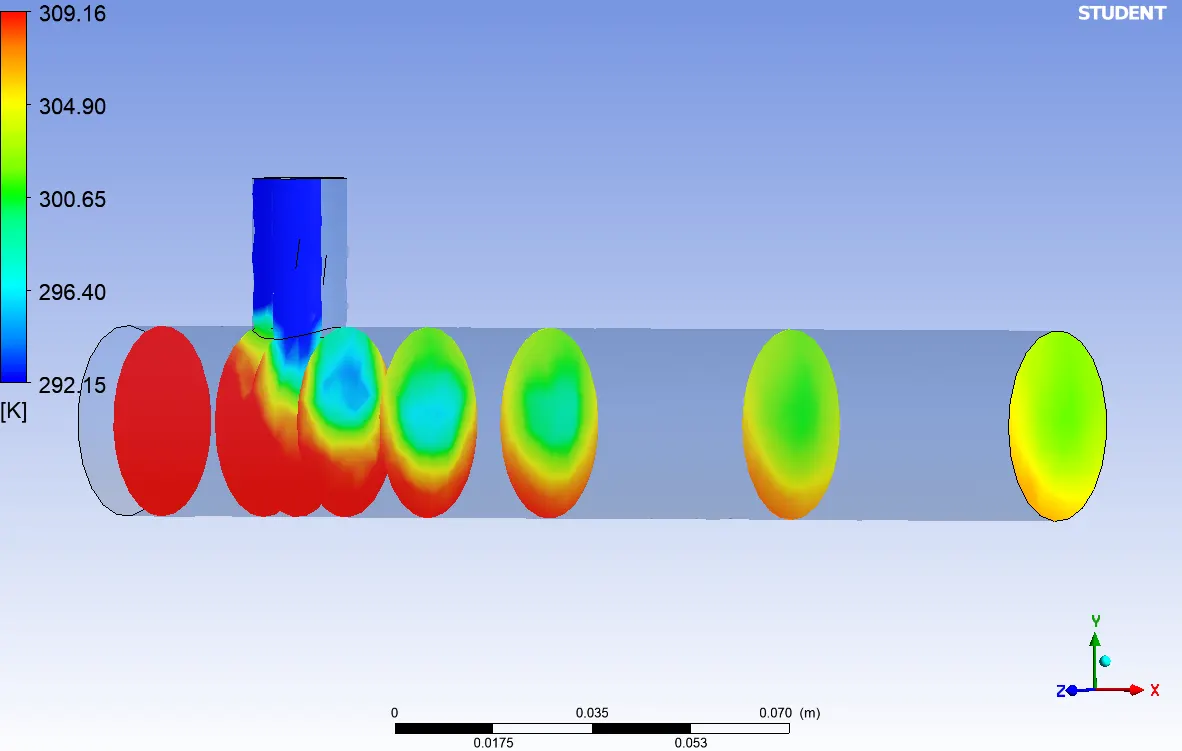
Mesh length 0.001:
Mesh:
 Set up:
Scaled residuals 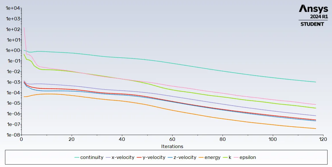
Area weighted average of outlet temperature 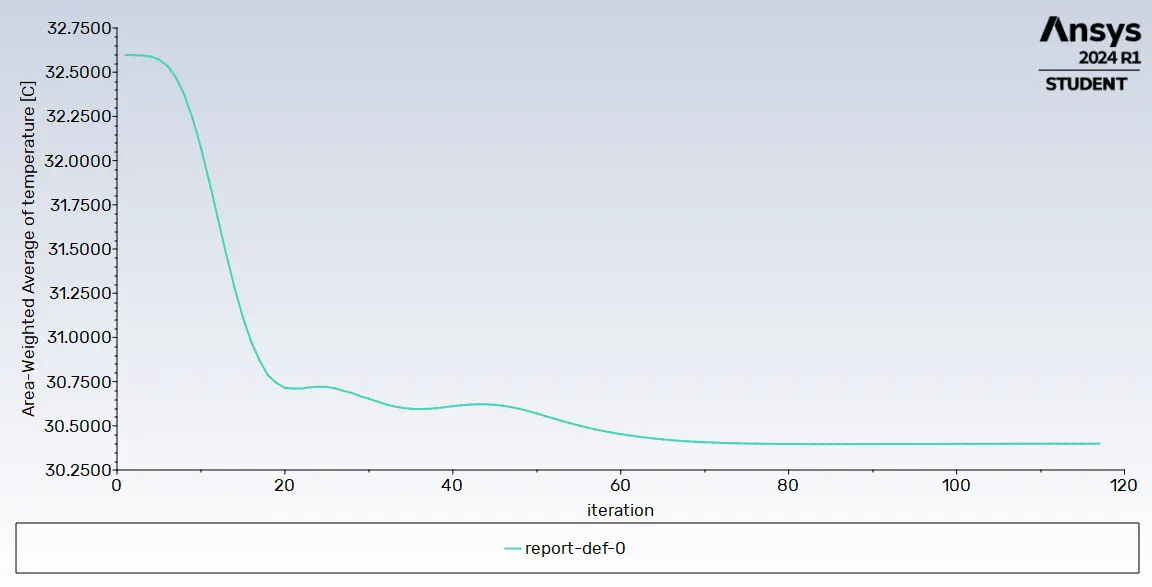 Standard deviation of outlet temperature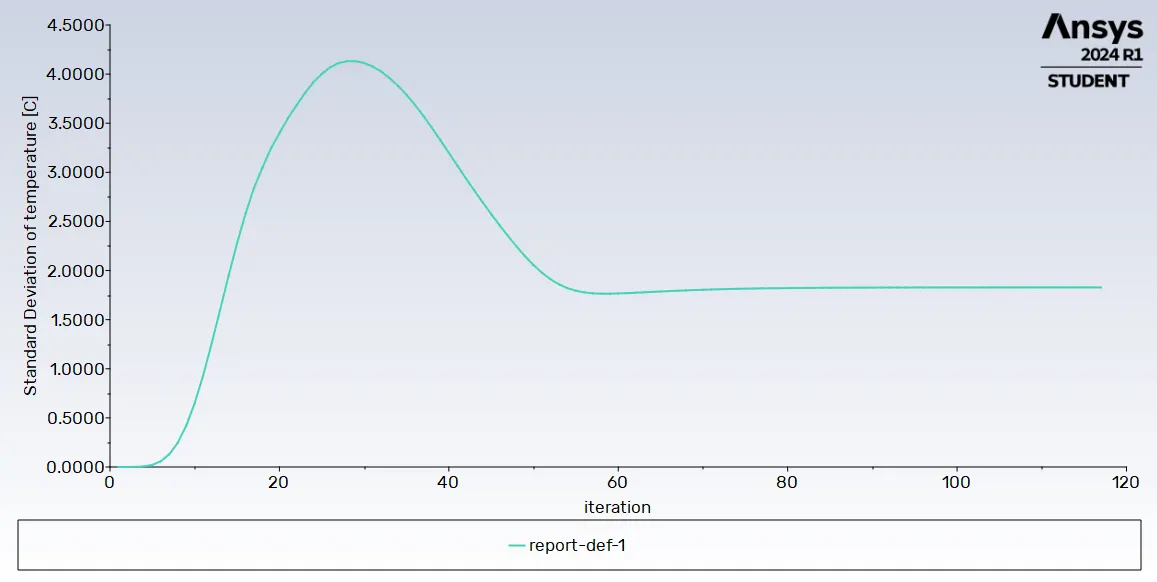
CFD Post:
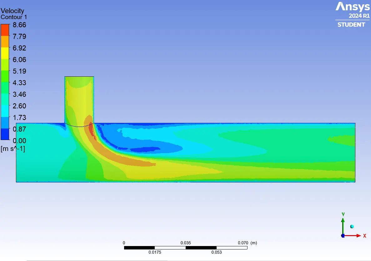
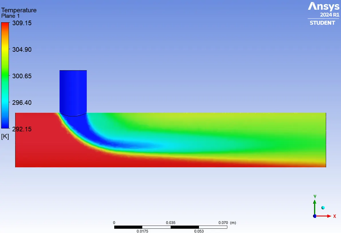 Velocity
 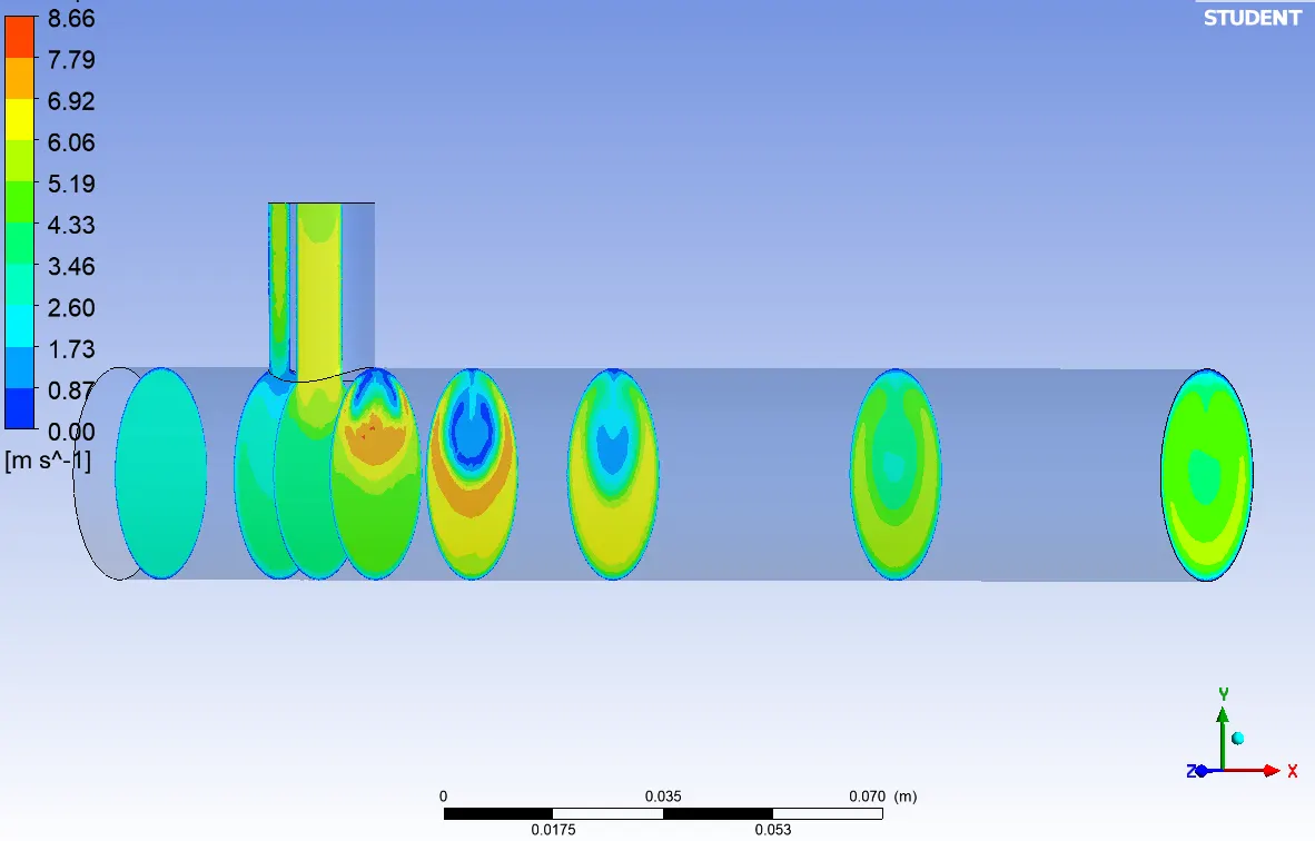 Temperature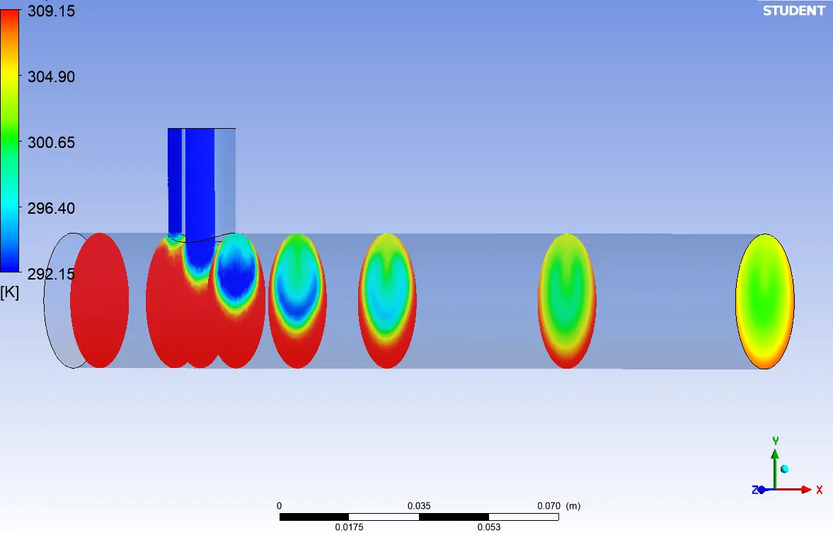
k epsilon, momentum ratio 4:
Mesh length 0.005 m:
Set up:
Scaled residuals:
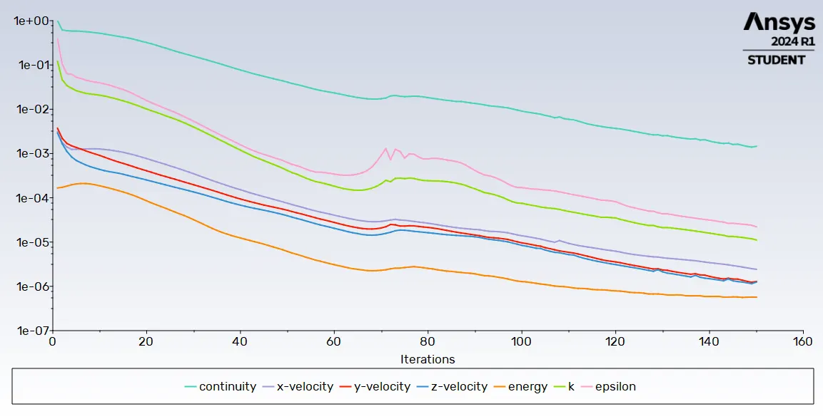 Area weighted average of outlet temperature
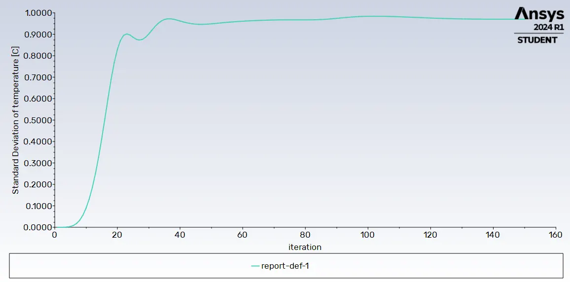
 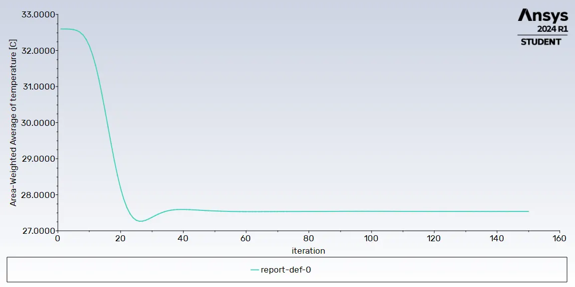 Standard deviation
  CFD Post: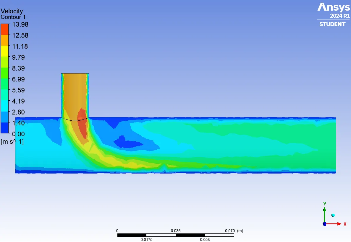
 Velocity
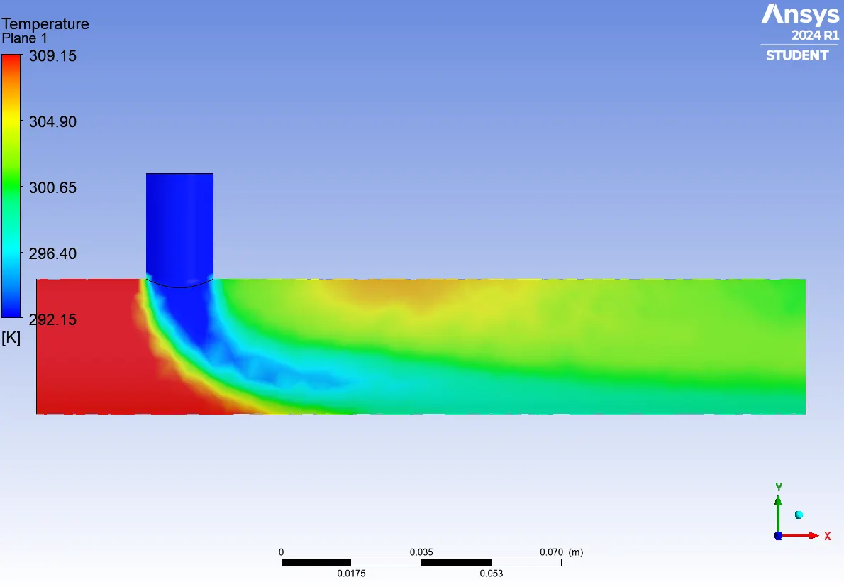
  Temperature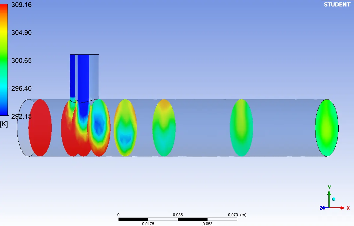
Mesh length 0.001:
Set up:
Scaled residuals:
 Area weighed average of outlet temperature
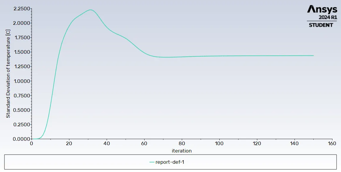
  Standard deviation
  CFD Post: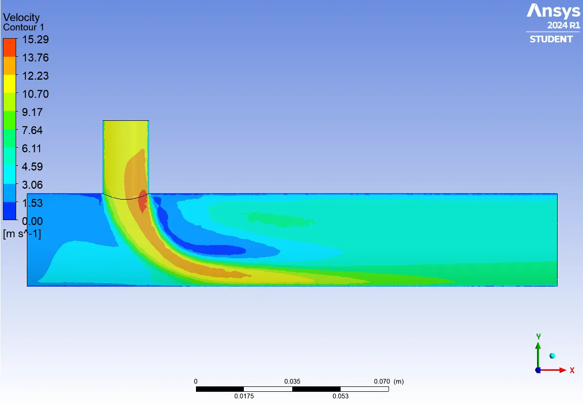
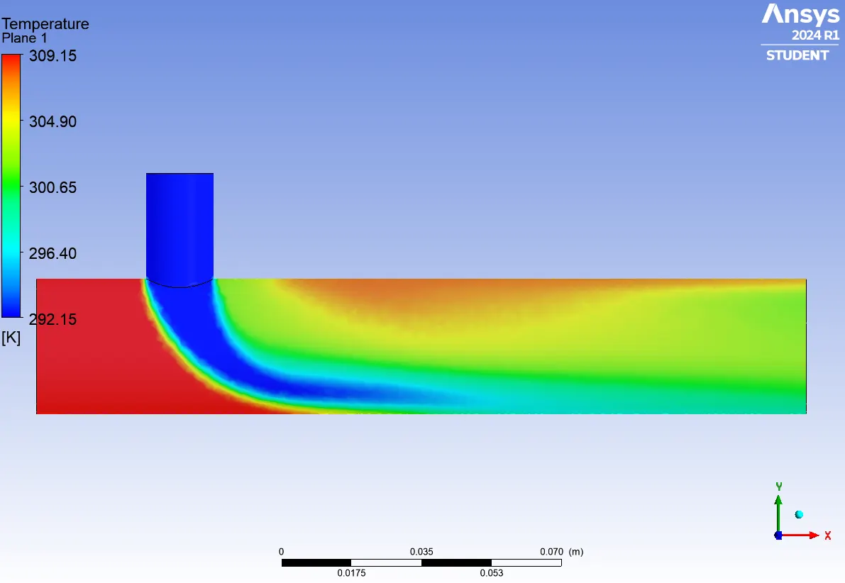 Velocity
 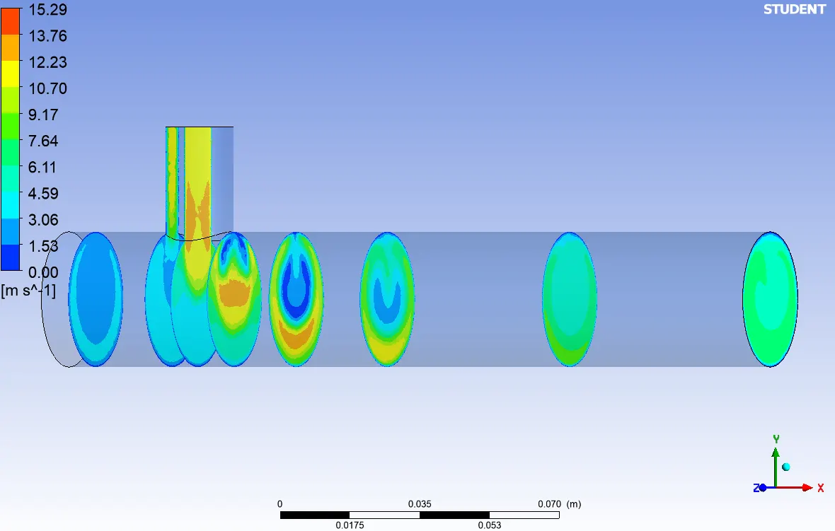 Temperature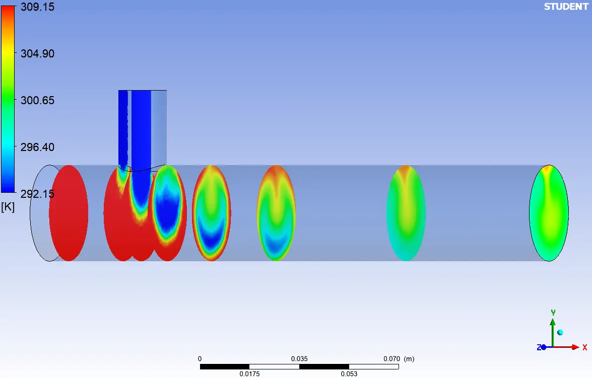
Conclusion:
In increase in length of the mixing Tee, the fluids are getting mixed well. Ends up in a more uniform temperature and velocity across the outlet. The Standard deviation of temperature at outlet temperature is greater for shorter pipe.
As the momentum ratio decreases, the scaled residuals fluctuate as the iterations proceed. The area-weighted average of outlet temperature is more when the momentum ratio is less. The standard deviation is more when the momentum ratio decreases. More uniform outlet temperature and velocity when the momentum ratio is greater.
From conducting the mesh-independent study, it is evident that the fines mesh gives better results. more uniform temperature distribution in the outlet.
Because of the non-slip condition, the velocity at the walls of the pipe is zero.
* Kindly refer the attached ansys file.