Week 1- Mixing Tee

Aim:-

Solving mixing tee by using ANSYS.

Objective:-

To set up steady-state simulations to compare the mixing effectiveness when hot inlet temperature is 360C & the Cold inlet is at 190C.

Use the k-epsilon and k-omega SST model for the first case and based on your judgment use the more suitable model for further cases. Giving the reason for choosing a suitable model is compulsory.

1. Case 1
   • Short mixing tee with a hot inlet velocity of 3m/s.
   • Momentum ratio of 2, 4.
2. Case 2
   • Long mixing tee with a hot inlet velocity of 3m/s.
   • Momentum ratio of 2, 4.

• For momentum ratio 2, the cold inlet velocity is 6m/s.
• For momentum ratio 4, the cold inlet velocity is 12m/s.

Procedure:-

Mixing tee is used in all over the world,since its misked two different fluid at a same time with a different temperature and different velocity to control the outlet the temperature.

K-EPSILON model-

• Two transport equations are also solved, one for turbulent kinetic energy (𝑘k) and the other for turbulent dissipation rate (𝜖ϵ). Here, 𝑘k still represents the turbulent kinetic energy, but 𝜖ϵ represents the rate at which turbulent kinetic energy is dissipated.
• Its suitable for high reynolds No.

K-OMEGA model:-

• Two transport equations are solved, one for turbulent kinetic energy (𝑘k) and the other for specific dissipation rate (𝜔ω). 𝑘k represents the energy associated with the turbulence, while 𝜔ω represents the rate at which turbulence dissipates.
• Its suitable for high & low reynolds No.

CASE 1 :- MIXING TEE SHORT

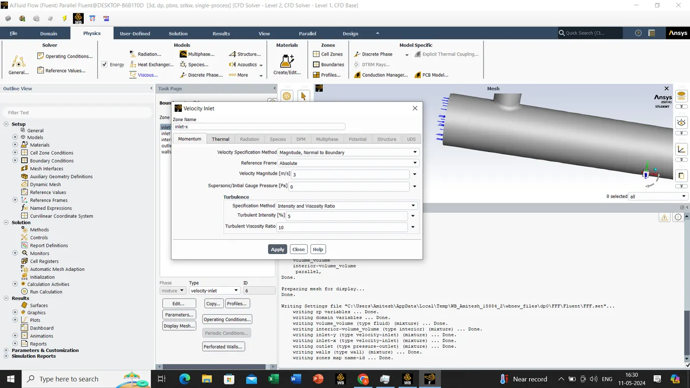
• Hot Inlet Velocity 3m/s.
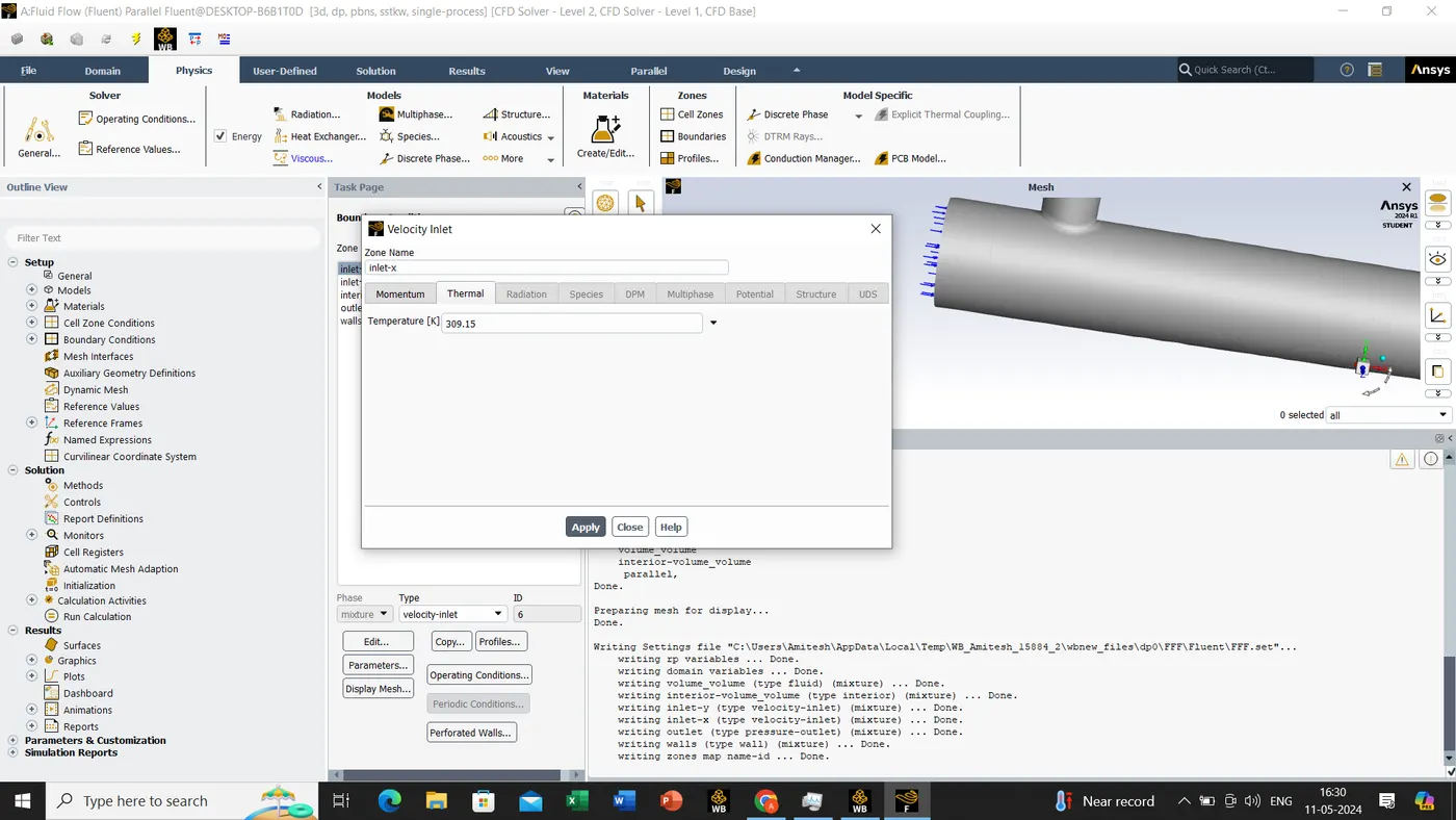
• Hot Temperature 36'C.
• Momentum Ratio 2.
• Cold Inlet Velocity 6m/s.
• Cold Temperature 19'C.
• Number Of Iteration 150.
• CASE 1 (K-EPSILON MODEL).

• We shall open the ANSYS software and later select the Fluid flow(fluent) & drag and down to the project schematic.

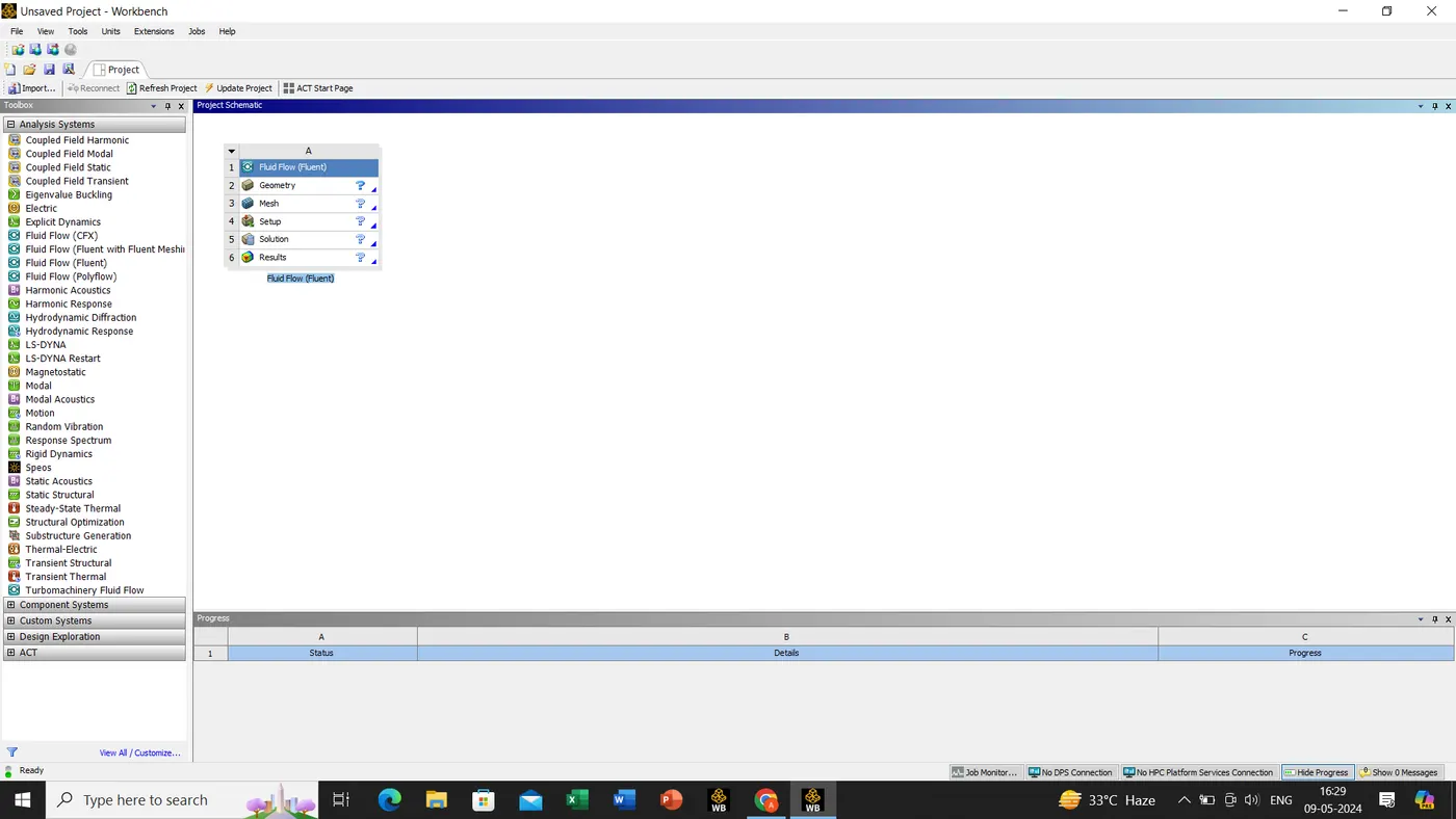
• Double click on the Geometry

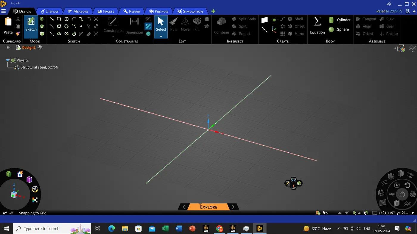
• Our first task is to import the geometry into spaceclaim to extract the fluid volume.
• Open Fluent workbench. Double click on geometry to open spaceclaim.
• Import the geometry by File>Open>file location.
• Once the file is opened we can extract the fluid volume.
• Go to prepare module and click extract volume.
• Select the edges of the two inlet and outlet using the edge selection option and click the green tick. The volume is generated.

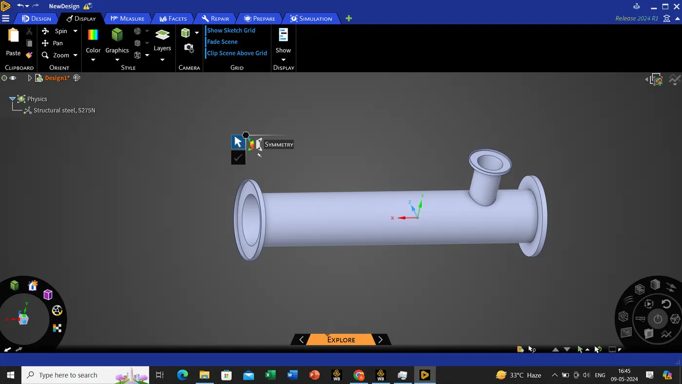
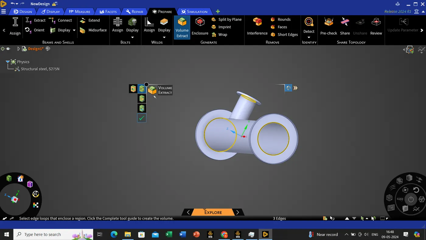
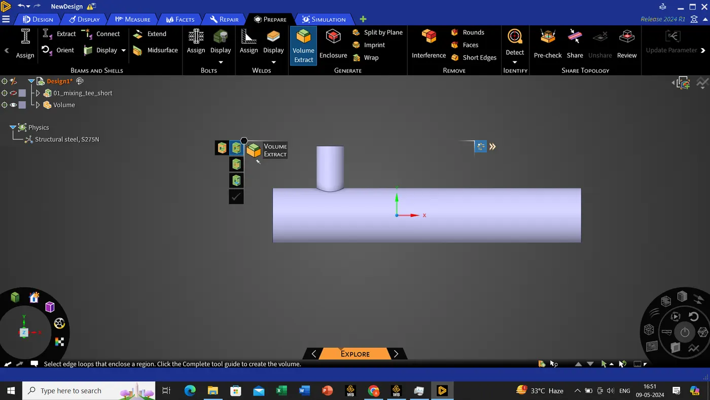
• Once the volume is extracted, we can exclude the body from simulation since we are concerned about the fluid flow happening inside the geometry.
• Right click on shell>select exclude from simulation. The body is now excluded from simulation.
• We can directly close the geometry without saving since its autosave.
• Next we can move onto the meshing process.
• Double click on the mesh in fluent workbench.
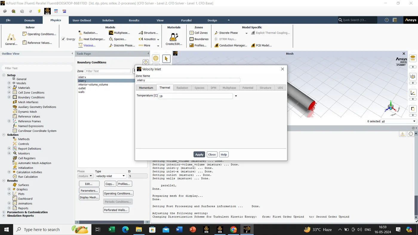
• Once the geometry is opened in the mesh module, before create a named selection we have to select the face as shown below.

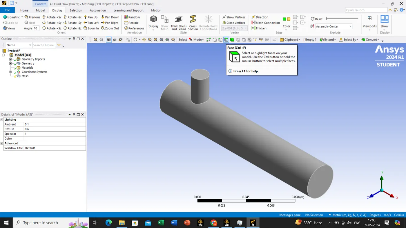
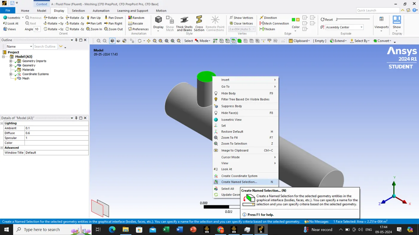
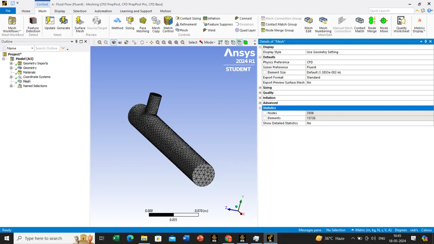
• Once the name has been done, we move to meshing, on left hand side we see the mesh in the project, click the right button and few options will appear later click on the generate mesh for the result as shown in below.

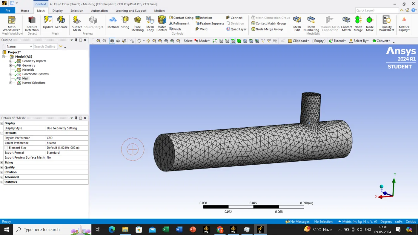
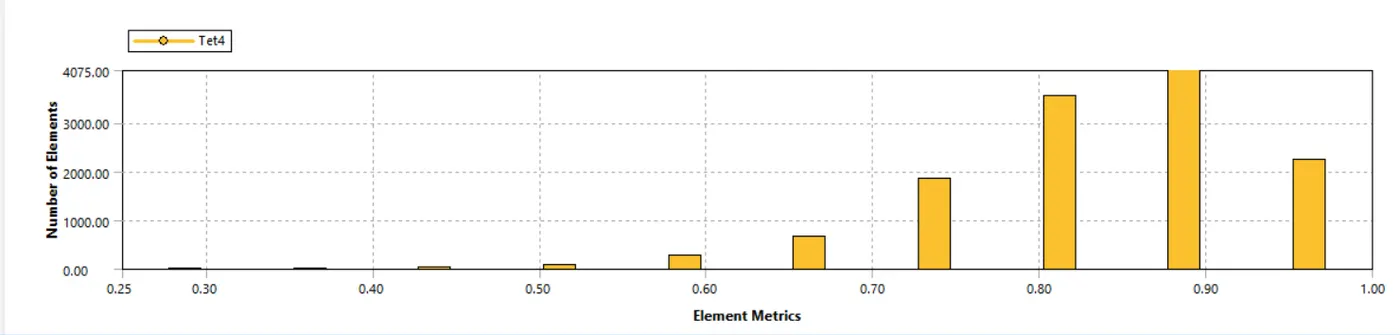
• As we can see on left hand side the ->details of mesh->Statistics->No of mesh nodes=2836 & No of mesh elements=12732

• The least quality element's element metrics value was higher than the 0.05 or 5% value, this explains that the mesh quality is good.

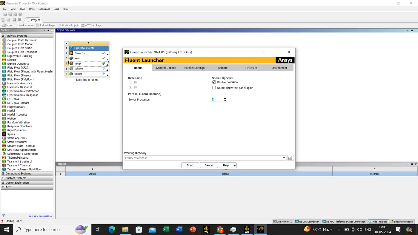
• Once the mesh is done we will move out and go for a setup, in solver options we had to select the double precision and in solver processor will go for 1 as per our cpu configuration.

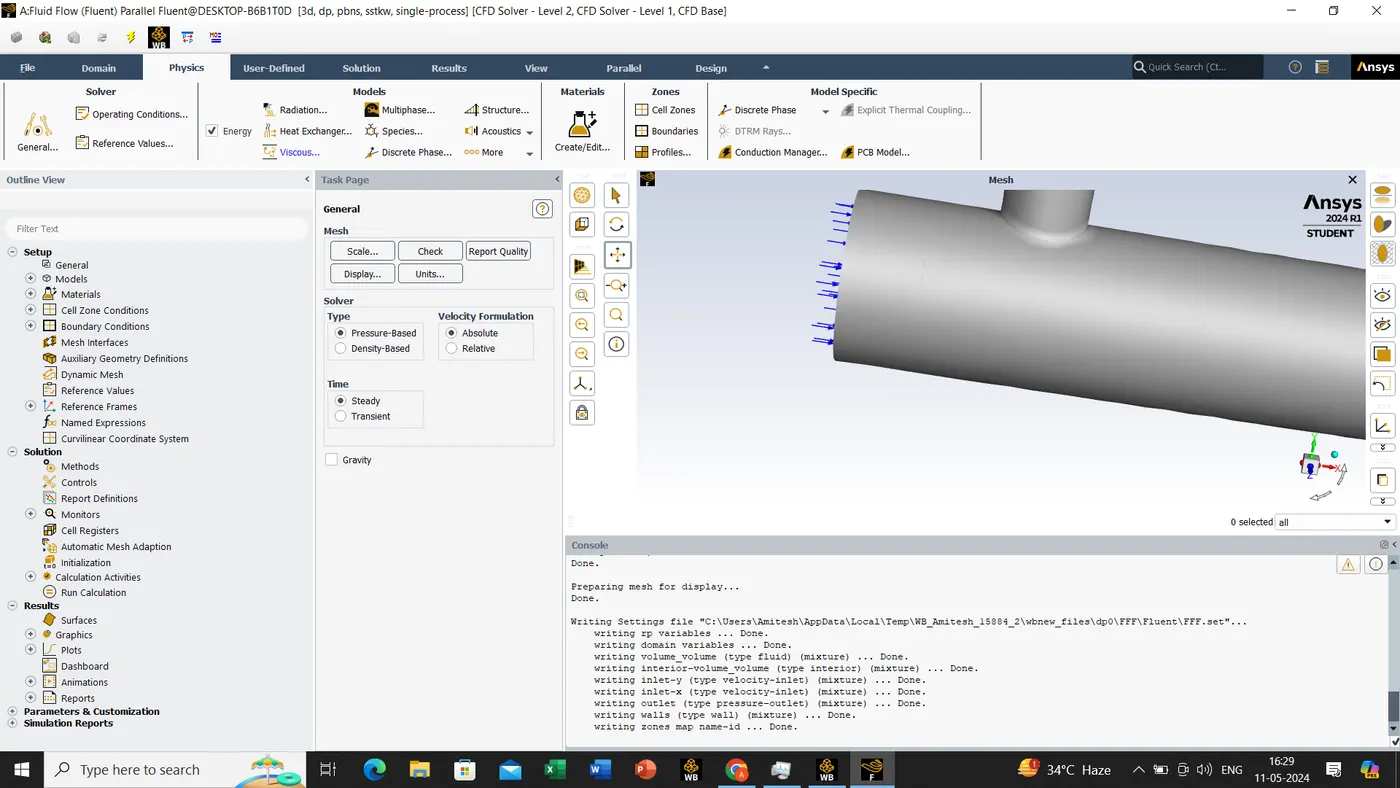
• Since once setup is launch we have to select the desire function to execute.
• Physics-> solver-> general-> select the type as pressure based & velocity formation as absolute & for the times as steady -> select the energy

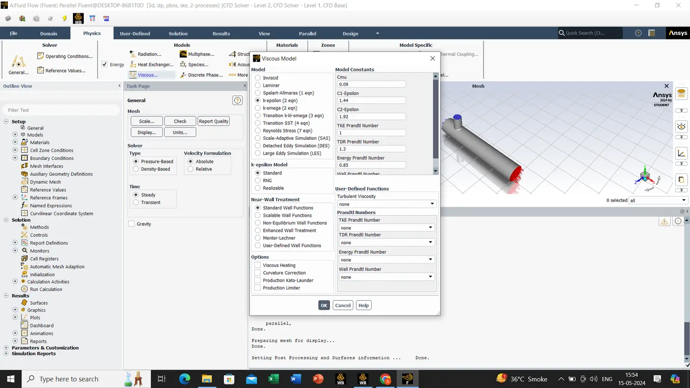
Since this is the case for K-epsilon, Physics-> Viscous-> select the case in which you had to simulate.

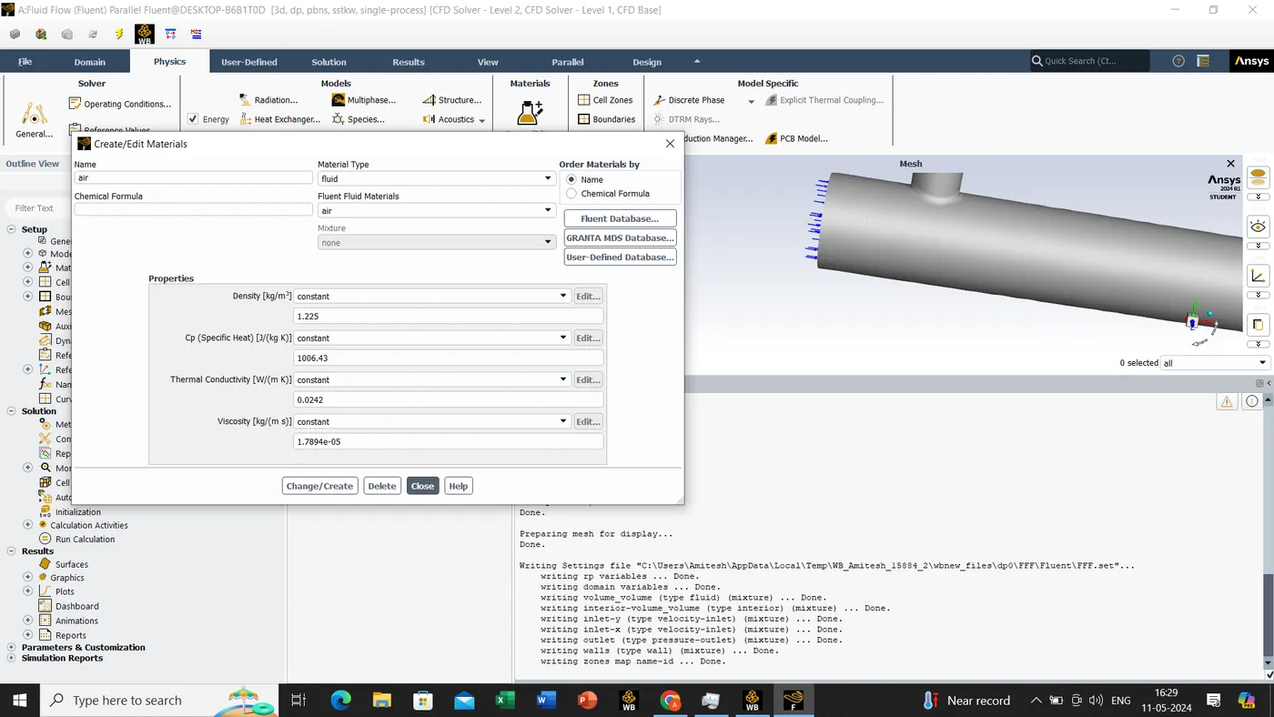
• Physics-> Material[for details as shown below]

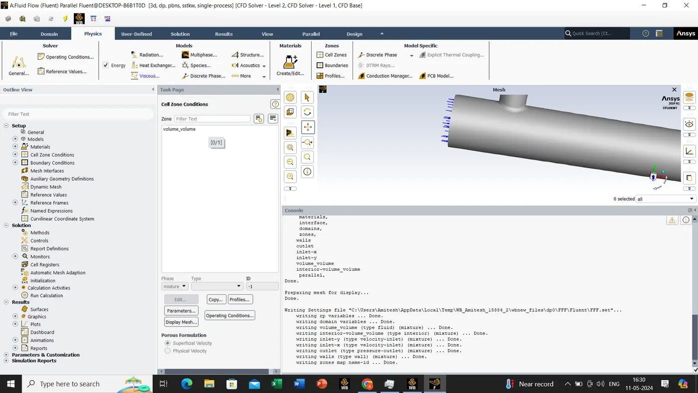
• Physics->Zones->cell zones[for details as shown below]

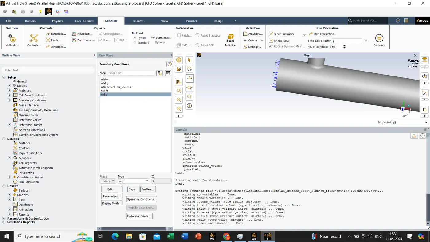
• Physics->Zones->Boundaries[for details as shown below]

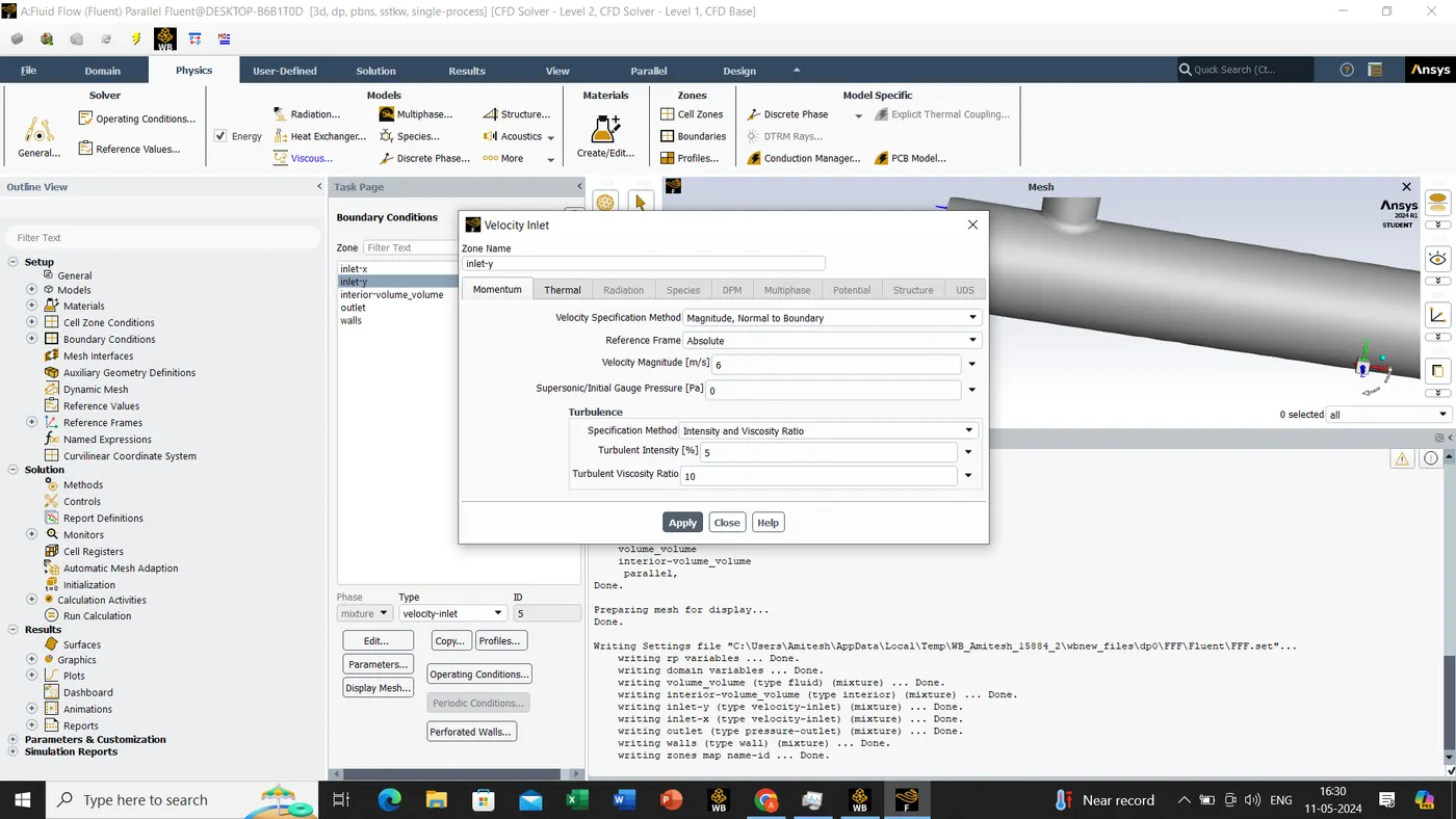
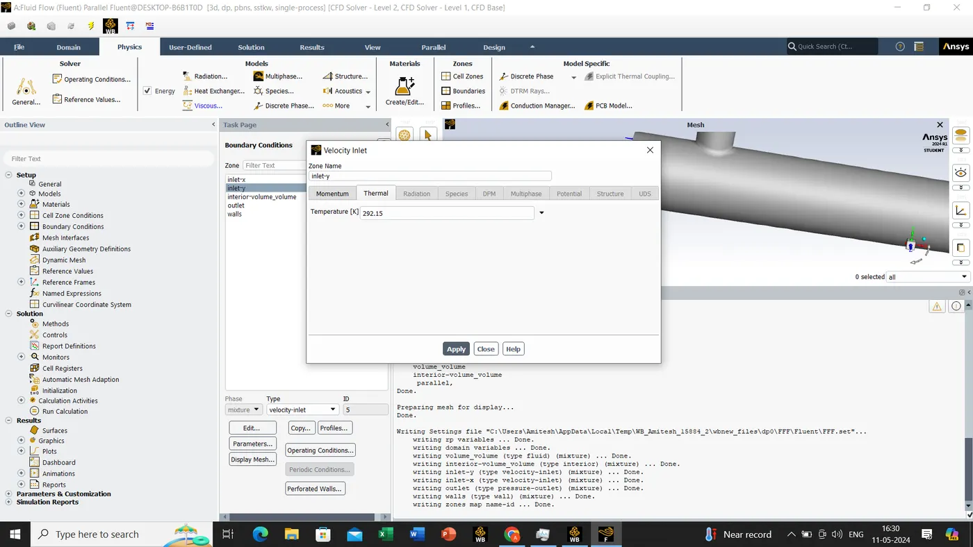
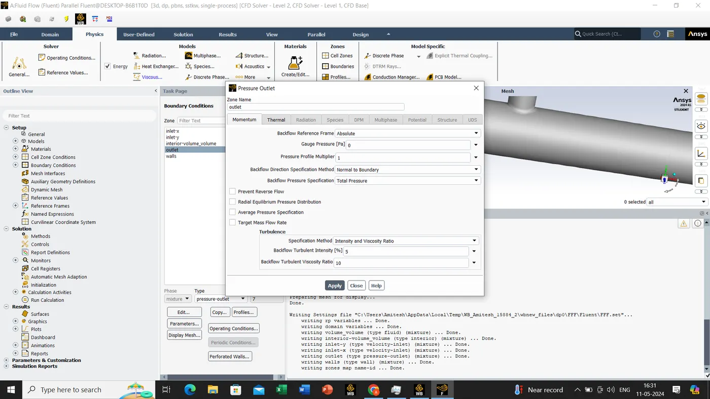
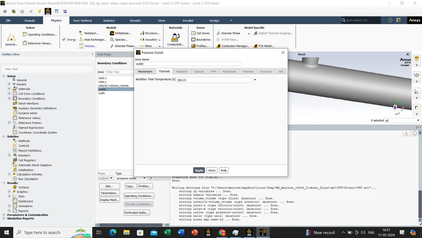
• For Solution-> method(hybrid)-> Click on t=0 for initialize -> Enter the no of iterations to run -> Calculate

Final results:-

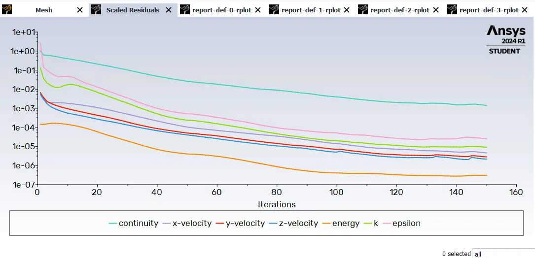
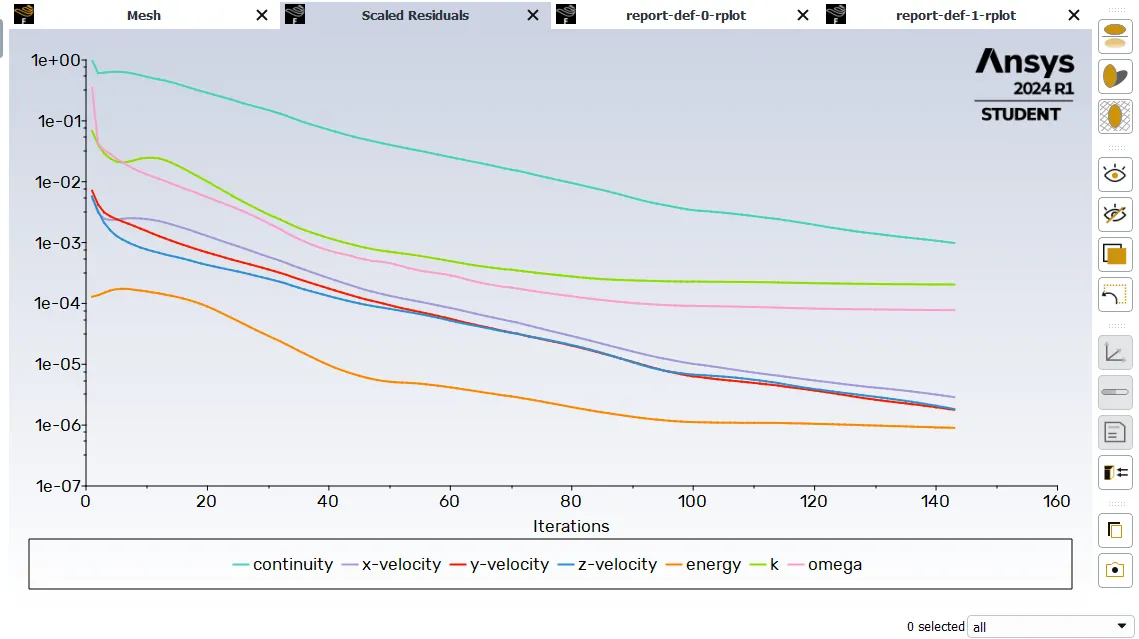
-> SCALED RESIDUALS

->AREA WEIGHTED AVERAGE OF PRESSURE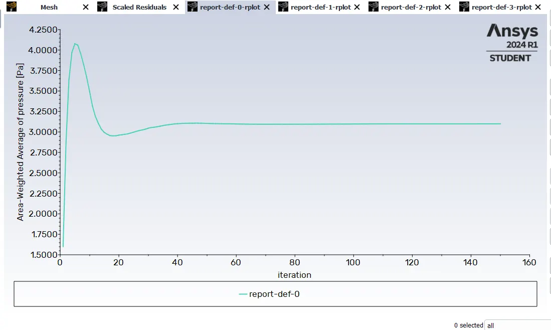

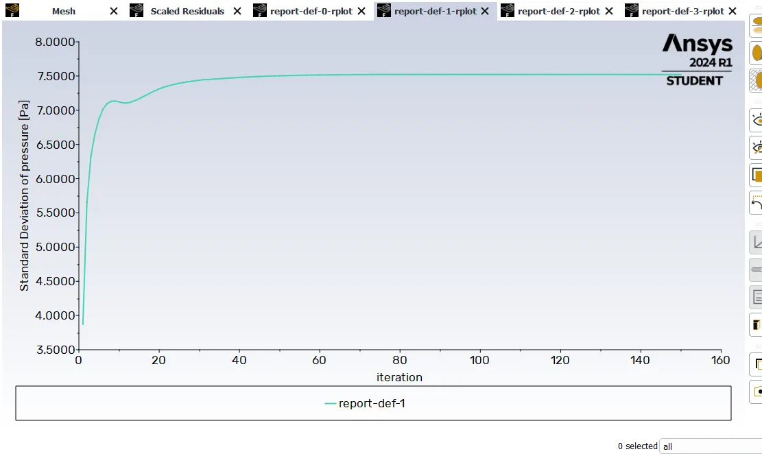
-> STANDARD DEVIATION OF PRESSURE

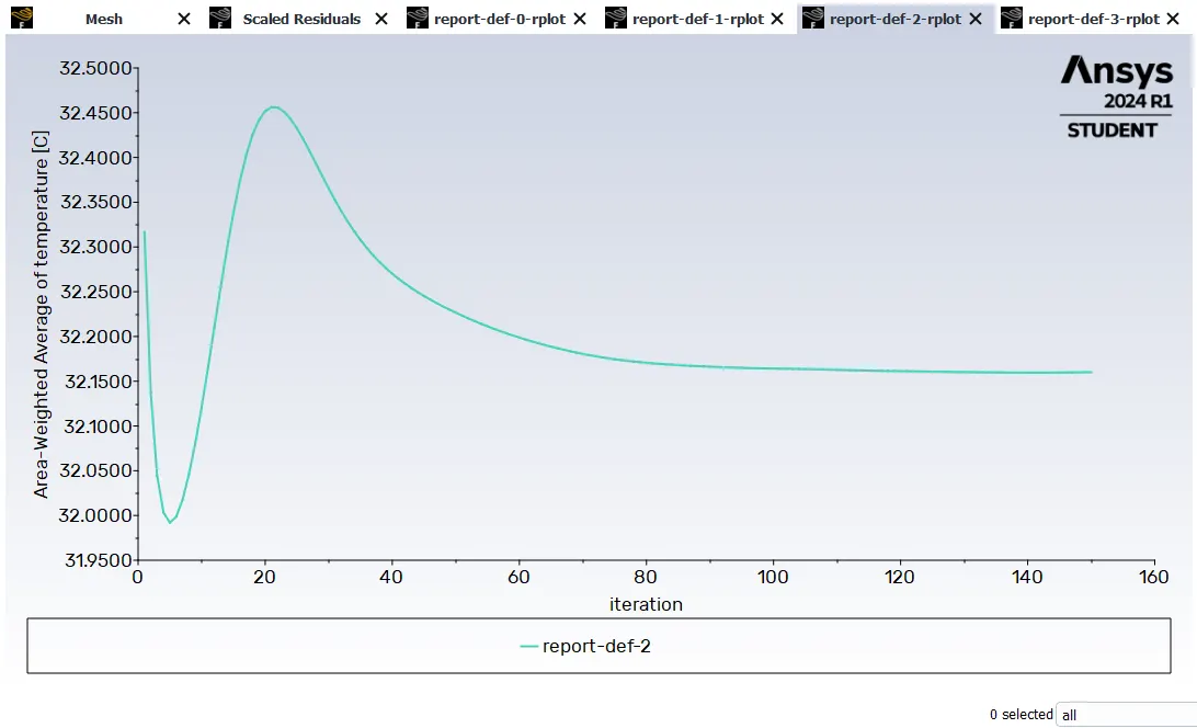
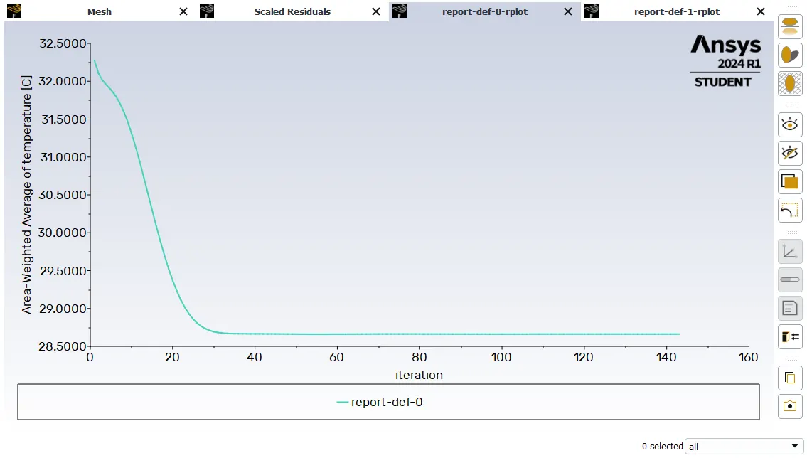
-> AREA WEIGHTED AVERAGE OF TEMPERATURE

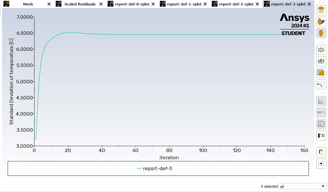
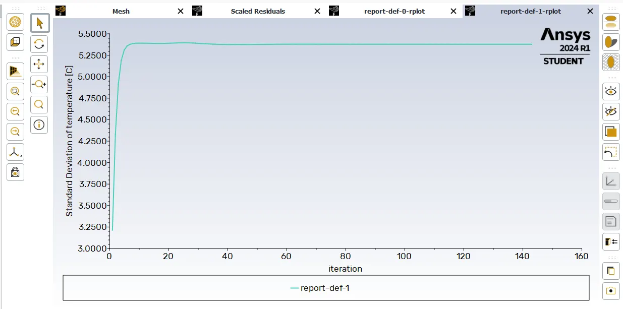
-> STANDARD DEVIATION OF TEMPERATURE

• Once we have done with this we will close the tab and return to the main tab i.e., ANSYS Workbench, we will double click to the result and the new final tab will be open.
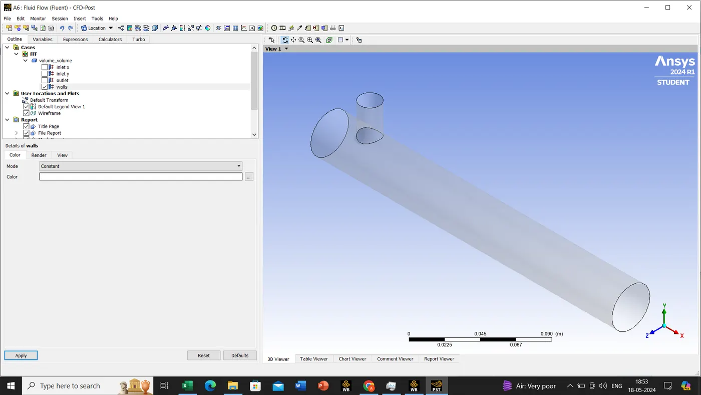
• Once the tab is open we will select the wall, which is the part of mixing tee.Once we will select the wall and double click to see its properties -> render -> Transparency value as per our choice
• Insert -> Location -> Plane (Plane 1)
• Plane 1 -> Geometry No changes -> Color -> Variable ( Select the velocity or temperature for showing the result in 3D viewer) -> Apply.
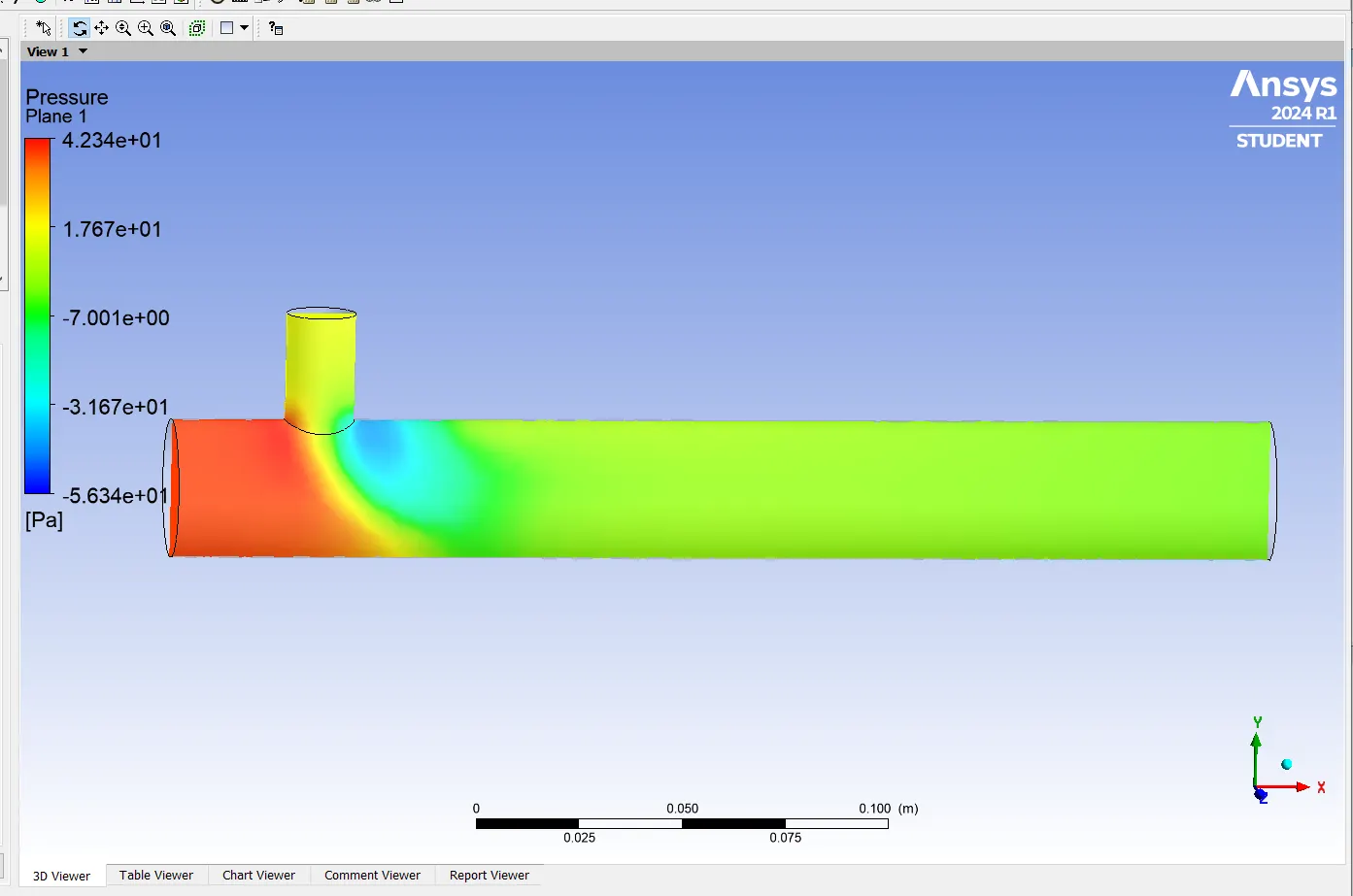
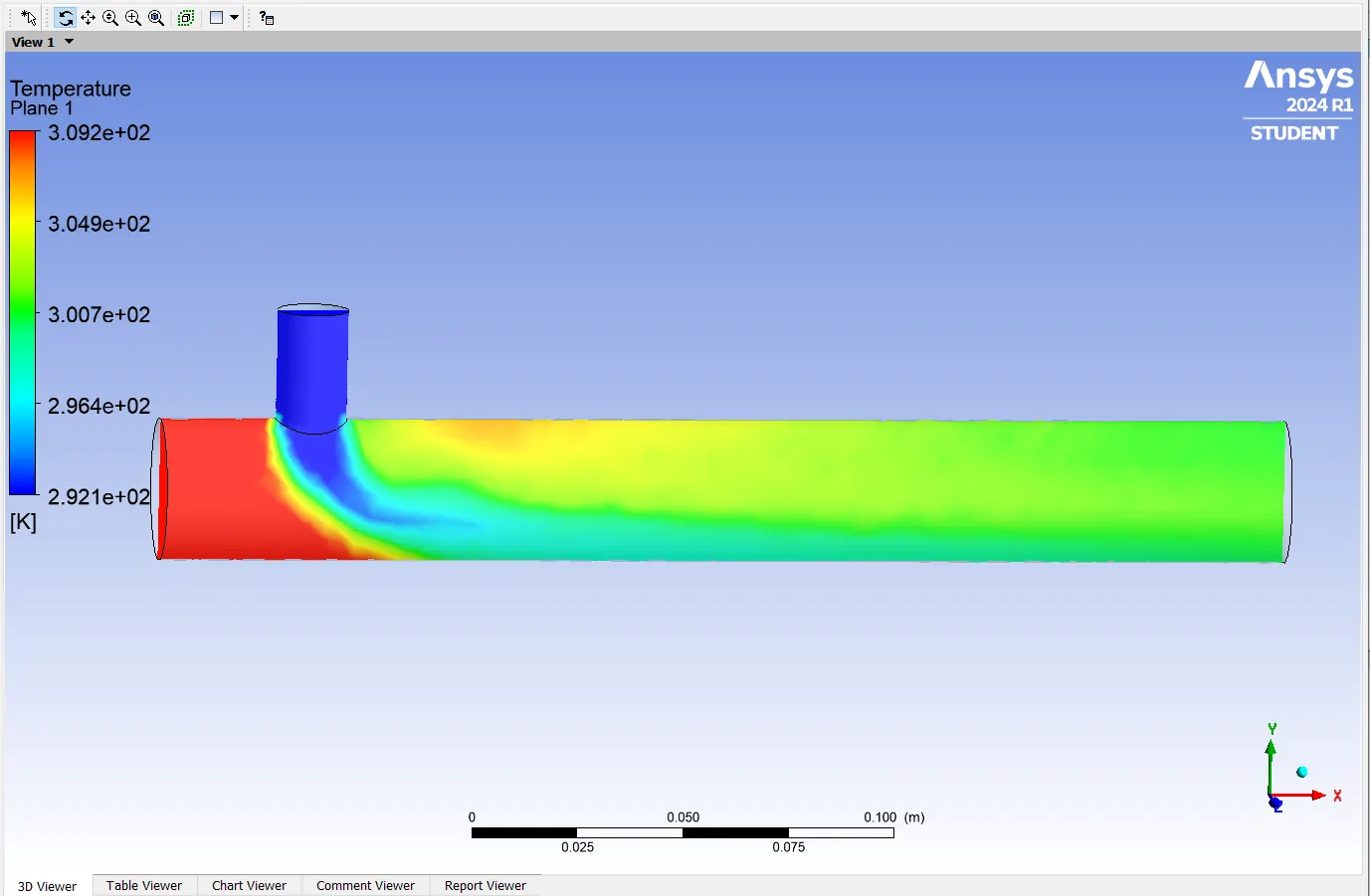
• Result for velocity and temperature.

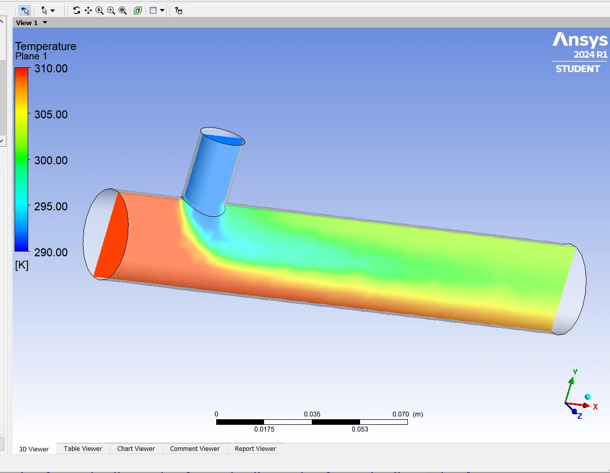
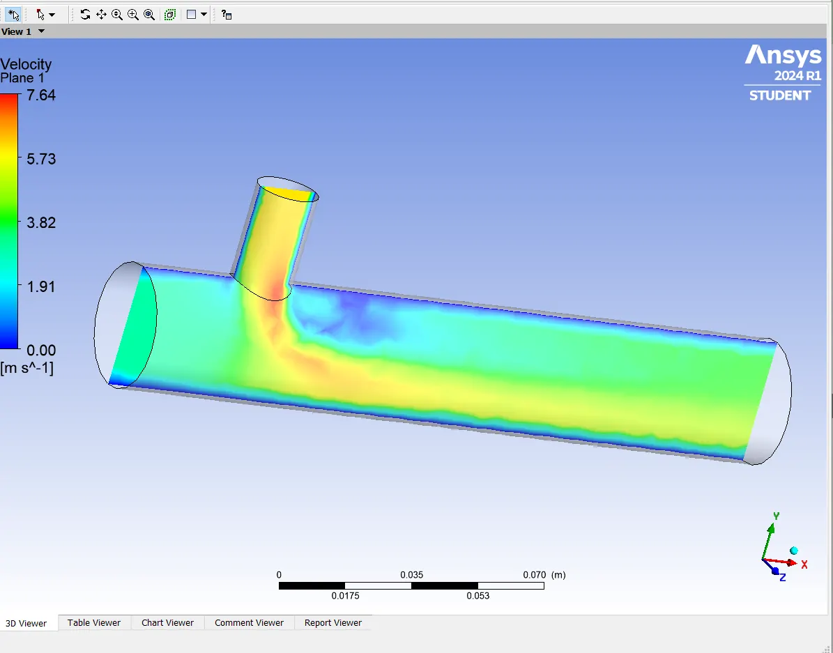
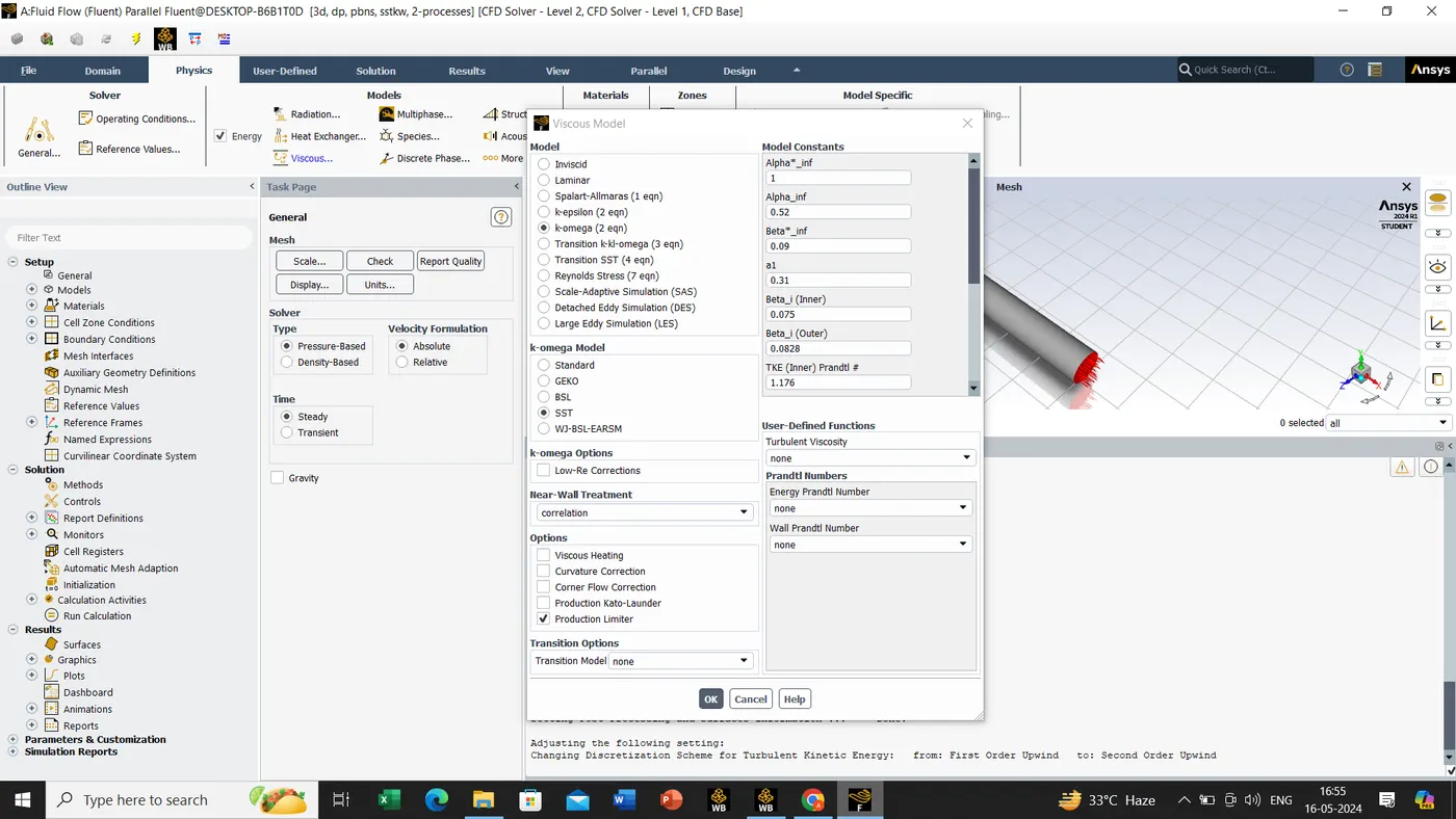
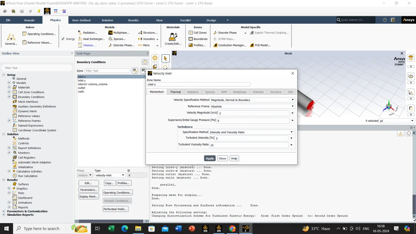
• Similary we will be doing for K-Omega as case 2, parameters are shown below,

• Hot Inlet Velocity 3m/s.
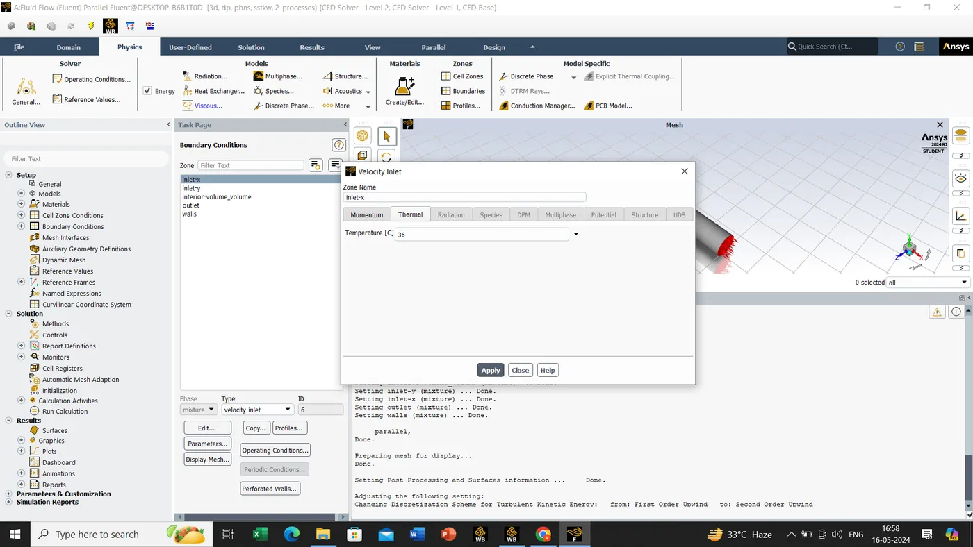
• Hot Temperature 36'C.
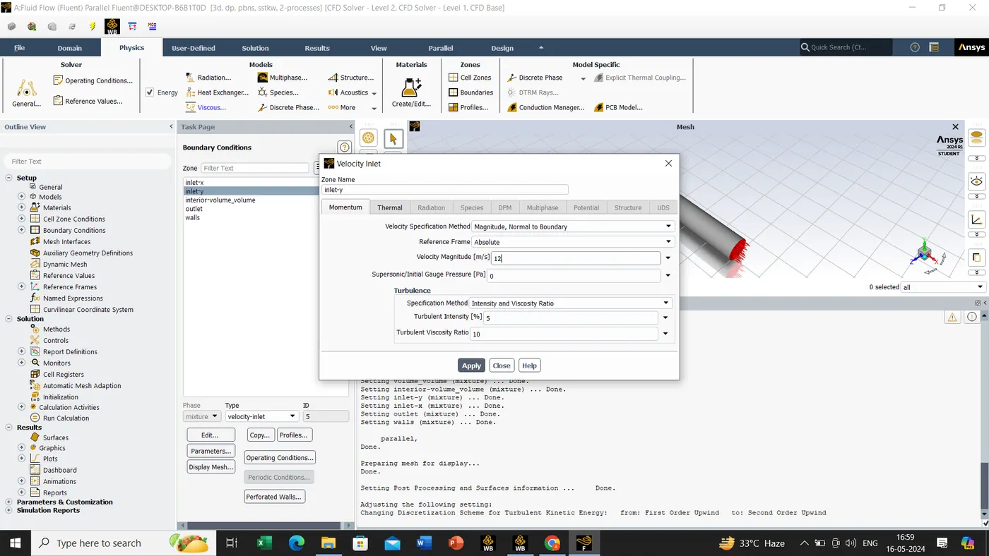
• Momentum Ratio 4.
• Cold Inlet Velocity 12m/s.
• Cold Temperature 19'C.
• Number Of Iteration 200.
• CASE 2 (K-OMEGA MODEL).

Now we will be doing same steps as discussed above for case 1, in this we will directly jumping to the setup which is present in the ANSYS workbench, the changes in any value will be shown for better understanding.

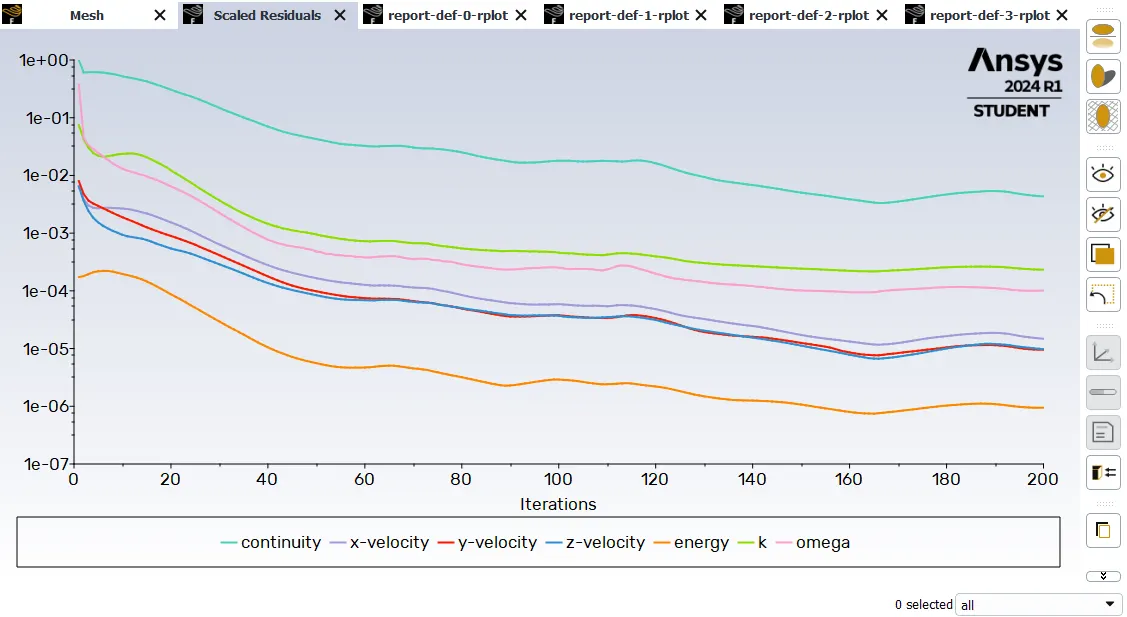
Final results:-

-> SCALED RESIDUALS

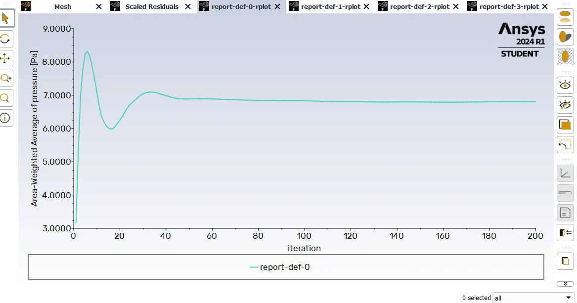
->AREA WEIGHTED AVERAGE OF PRESSURE

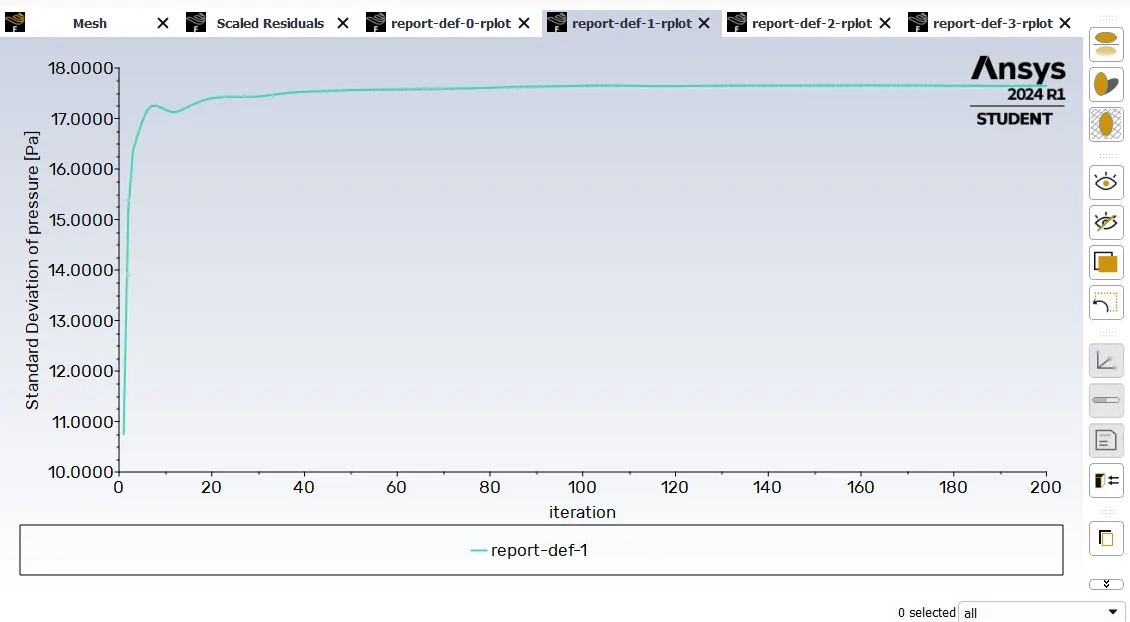
-> STANDARD DEVIATION OF PRESSURE

->AREA WEIGHTED AVERAGE OF TEMPERATURE

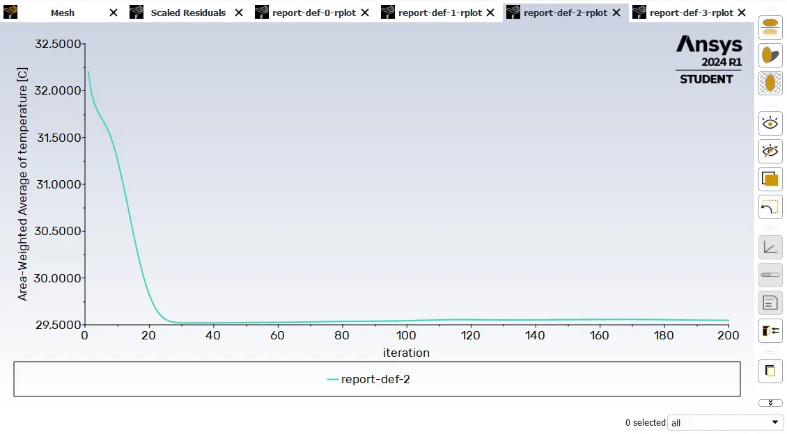
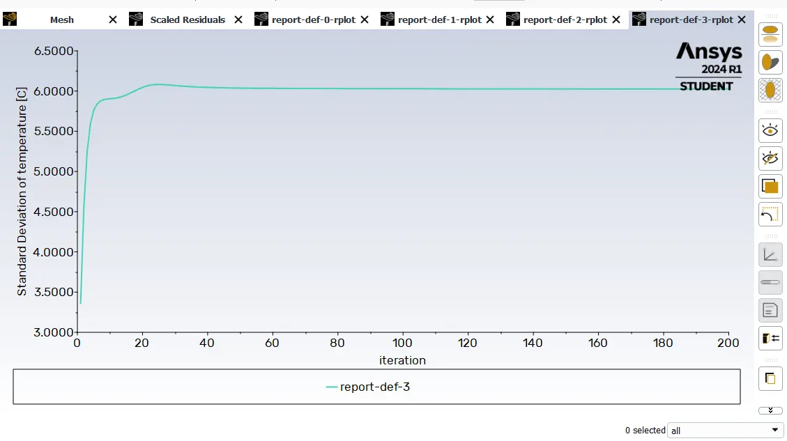
-> STANDARD DEVIATION OF TEMPERATURE

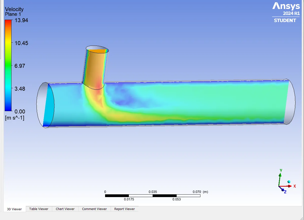
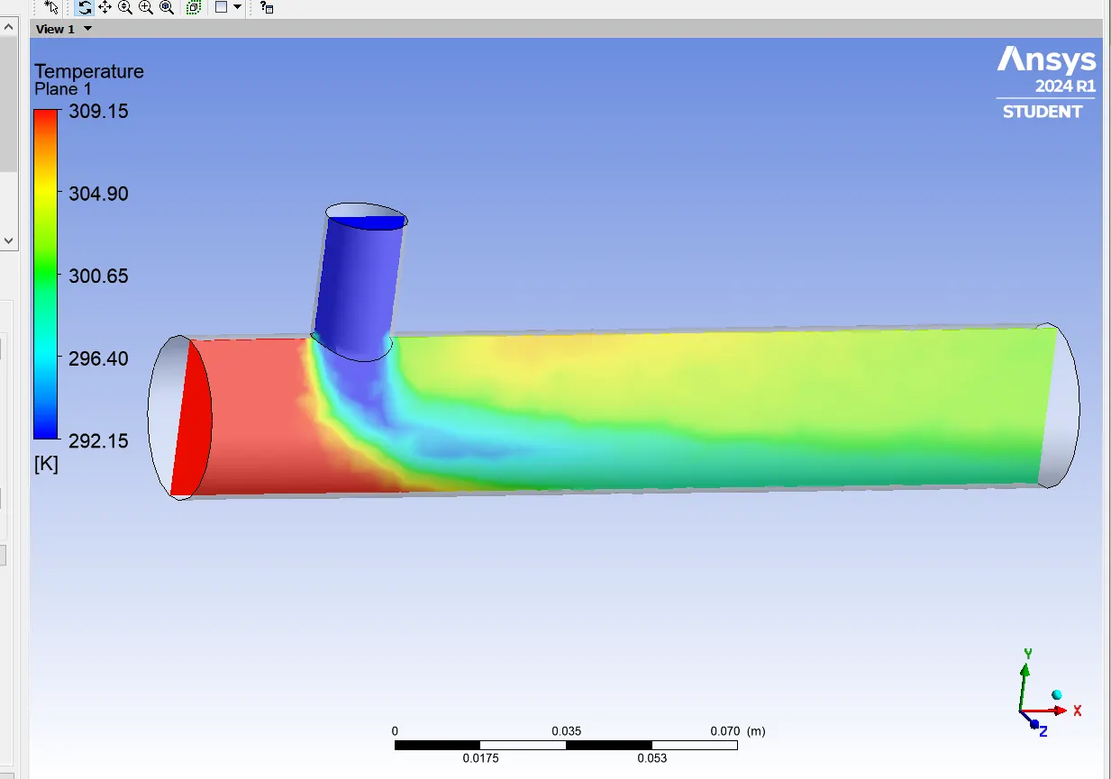
• Result for velocity and temperature.

Now we will be solving for long mixing tee considering the same case 1 and case 2, lets go ahead with the case 1.

CASE 1 :- MIXING TEE LONG

• Hot Inlet Velocity 3m/s.
• Hot Temperature 36'C.
• Momentum Ratio 2.
• Cold Inlet Velocity 6m/s.
• Cold Temperature 19'C.
• Number Of Iteration 150.
• CASE 1 (K-EPSILON MODEL).

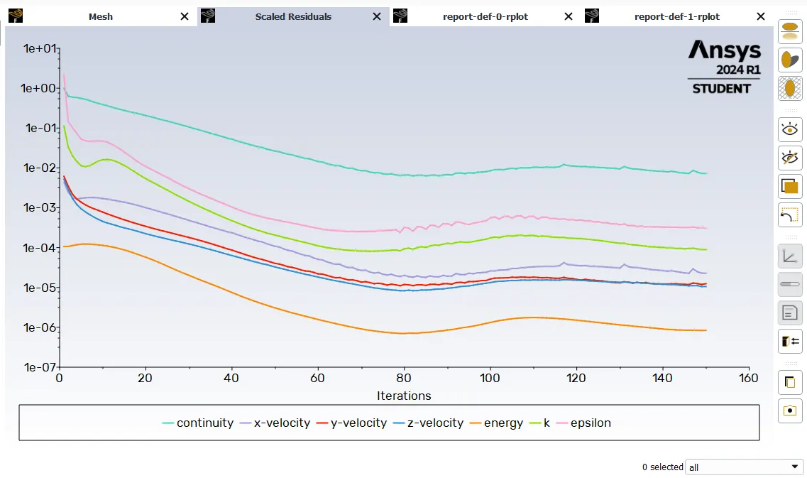
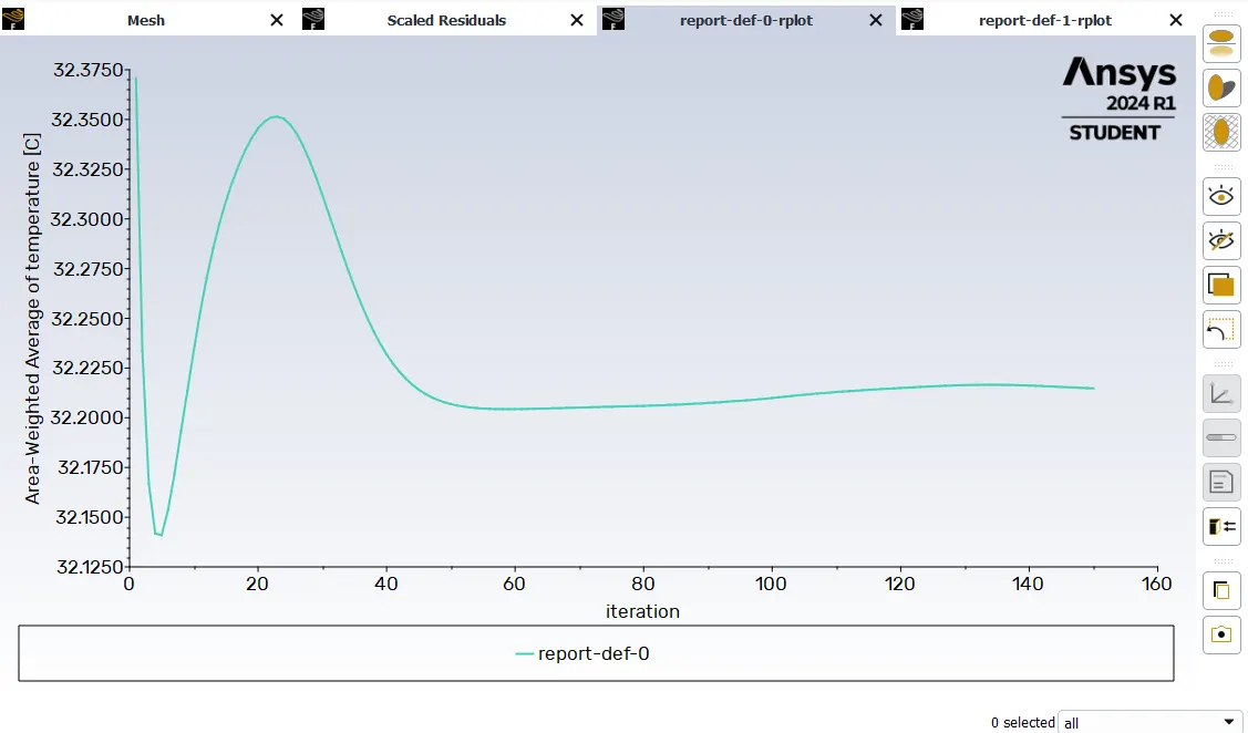
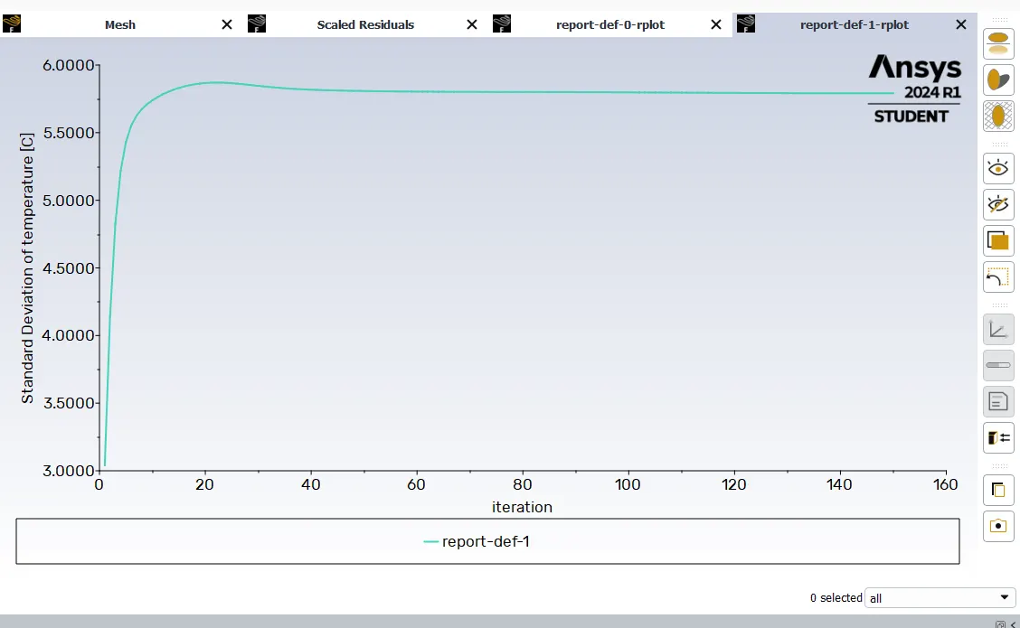
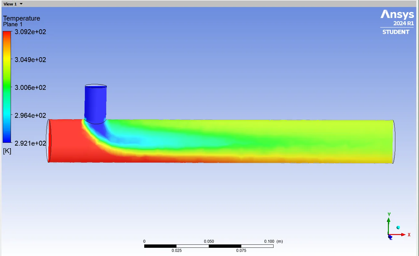
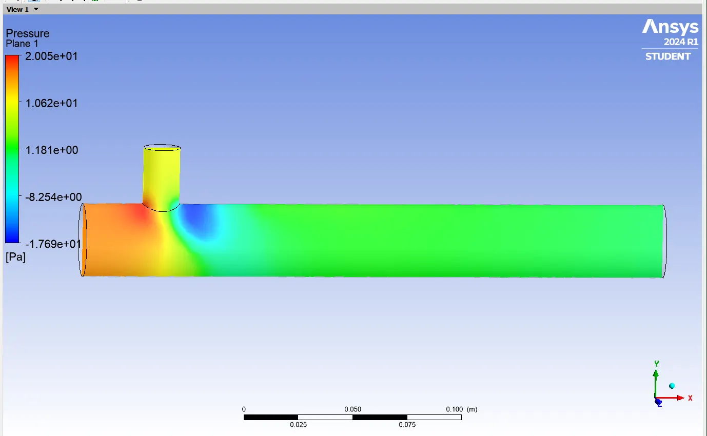
• Similary, we will be doing for K-Omega as case 2, parameters are shown below,

Case:-2

• Hot Inlet Velocity 3m/s.
• Hot Temperature 36'C.
• Momentum Ratio 4.
• Cold Inlet Velocity 12m/s.
• Cold Temperature 19'C.
• Number Of Iteration 200.
• CASE 2 (K-OMEGA MODEL).

Since we are considering our working fluid as air, density(rho) is 1.225 kg/m.

we have the formula,

T(mix)=m(hot)*T(hot)+m(cold)*T(cold)/m(hot)+m(cold)

where,

T(mix)= AVG Temperature of fluid at outlet

m= Mass flow rate of fluid=rho*A*V

V=velocity

A=Area

T= Temperature

T(h)=36C ; T(c)=19C

V(h)=3 m/s ; V(c)=6 m/s

A(h)=891.86 mm^2 ; A(c)=221.42 mm^2

m(h)=3277.58 kg/s ; m(c)=1627.43 kg/s

Substitute all values in above formula,

T(mix)=30.35C

we shall be doing for all as same as above.

	K-Epilson	K-Omega	K-Epilson	K-Omega
	M.R=2	M.R=4	M.R=2	M.R=4
No of mesh Nodes	2836	2836	3506	3506
No of mesh Elements	12732	12732	15726	15726
AVG Temp Outlet	32.47 C	32.4 C	32.7	32.27 C
STD Deviation of Temp	6.5 C	6.1 C	5.8 C	5.4 C
NO of Iterations	150	200	150	200