Week 1- Mixing Tee

In this challenge, there are two mixing tee is here, so first we started with short mixing tee. First we opened workbench then we opened fluid fluent then we opened spaceclaim, in spaceclaim we import the geometry, so previously we discussed we started with short mixing tee. after import the geometry we started the geometry clean up. in this short mixing tee we need wall where the heat flux will flow through the body wall. so we seen some surface which one we no need for future activity. then we started to delete those parts. so it will be time consuming process.then we taken option called volume extract, in volume extract we choose edge's after we selected three edges then in down one right mark is there we selected then we seen left corner of tee one more new object added, then we hide the solid component. after that we don't need the solid component in mesh generation process so we did suppress for physics.

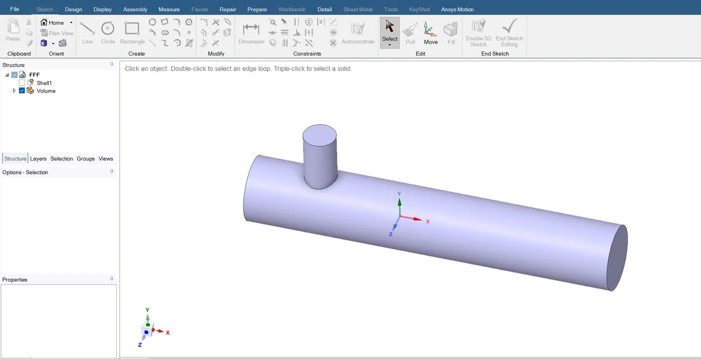
In this challenge we have two case.

1)case-1

• Short mixing tee with a hot inlet velocity of 3m/s.
• Momentum ratio of 2, 4.

2)case-2

• Long mixing tee with a hot inlet velocity of 3m/s.
• Momentum ratio of 2, 4.

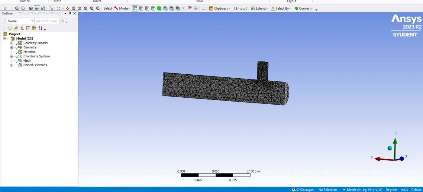
In case 1 there are two momentum ratio is there, so first we started with momentum 2.after cad cleanup we started with meshing, in meshing we started with face selection, then we started first selection that will be x-inlet, then second one y-inlet, then 3rd one outlet and last one wall.after selection of face we select the mesh then we started the mesh by default of sizing mesh. after that we got meshing of the body and good element number of count.

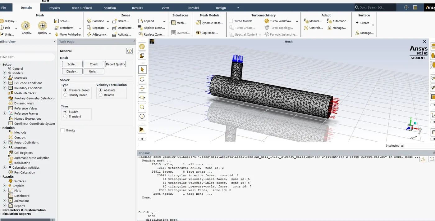
After completing of meshing we started the setup, in setup we selected solver option double precision and parallel simulation and we taken 4 processer then we putted ok. after opening more information printed out automatically.then we gone to the graphics window we seen geometry was there.then we started with mesh checking.then we got our mesh is okay.then we are going to next setting up physics. in this case we taking steady state solver then for small mach number flow we taken pressure-based solver then for velocity formulation absoulte option. then we are interested for solving temperature so we are using energy equation.so in this particular model the flow can be turbulent so that we are using viscous model then we are using k-epsilon model, after that we are using realizable k-epsilon model, then we selected standard wall functions.after we started add material, in add material we seen default one is there air, so we gone through air flow.after that we assign boundary condiation then we are selecting cell zone, in cell zone condiation we are selecting volume then we seen the intenal volume type is fluid.then we going for next one that is boundary then in boundary condiation we are selecting inlet-x , then we seen type is automatically set for velocity-inlet, then we selecting edit then our along inlet face my velocity is 3 m/s.after that incoming hot temperature along the pipe is 360C.then next we are going another velocity inlet that will be our y-axis, where my velocity inlet is 6m/s and my inlet cold temperature is 190C.

Then next we are going for soving part, in that one we want know what is our oulet temperature, so for that one we clicking in defination then we are interested in computing area weighted average and variable looking for that temperature then we need faces that will be our outlet then we createing report file and report plot and this is done for every iteration then we clicking ok.in this problem we are doing mixing problem, for understand the effectiveness of mixing so we need standard deviation and the variable is temperature and the face is outlet then we can create a another report file and another report plot for that one.once we complete the initial condiation, boundary condiation and material property, then next we are going for initialize the solution.in initialization we are using hybrid initialization then we click the initialize after ten iteration the initialization is done.

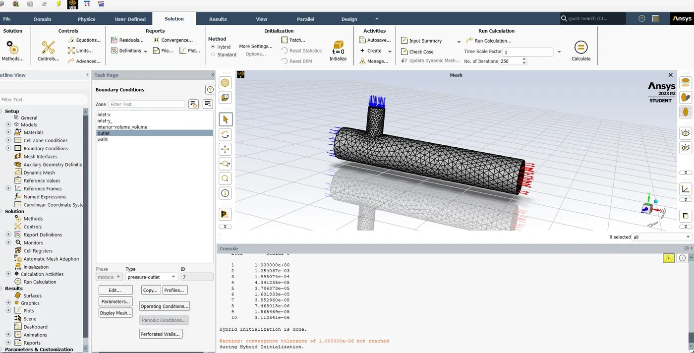
Then next we are ready for run the solver so we re running for 200 iteration.then we got the result.first we started we with scale residuals.

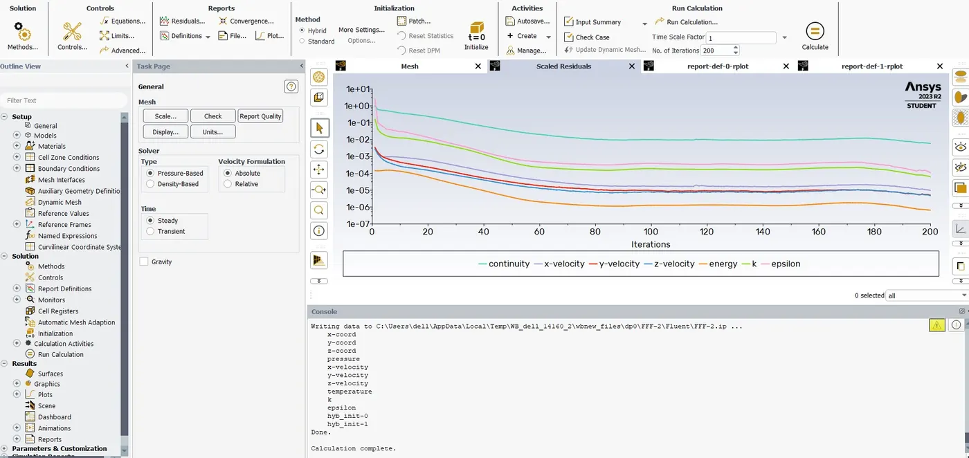
Here the no. of iteration continue the function have been calculated is close to zero. so here we can see that our continuity equation keeping in drcreasing.

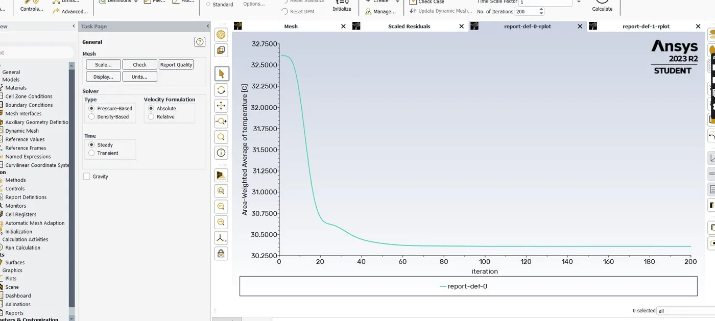
Here we can see that our area weighted temperature is arround 30.350C after that its contineously steady state flow.

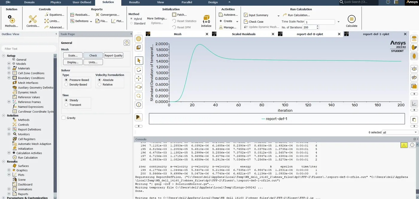
Here we can see that standard deviation of temperature in mixing point is going for highest point then its going uniformly.

Next we are going for post process the results, so we double click on results after that we can able see our model then we are enable our component we need only our walls, in wall after double clicking then we clicking in rendering then we are applying some transparency. so we need velocity and pressure disturbution. so for that we need to creating a plane xy- plane where the z value is zero.then we got our plane is exactly right in the middle.then we change to that one colour white. after that we can go to plane and then we did colour this one by a variable then we change to temperature then we apply. after we got result then we need bit more changes in range to user specified then we given minmum value of 190C and maximum given as 360C then apply so we seen legend was changed. after that we gone for default legend view then gone to apperance then text parameter to fixed point rotation then its may be 2 decimal places then apply. so we got a good legend view.

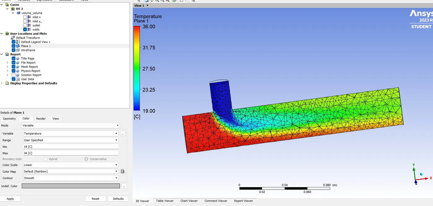
In this first case we used k-epsilon model short mixing tee with a hot inlet velocity 3m/s and momentum ratio 2 taken, so we got good output and good mixing path.next one we taken same value but we changed only k-omega SST model.

In next case directly we started with setup, after opening of setup we opened the viscous model then we are using here k-omega SST model. then we checked our all input value is there so i directly gone for solving part,then next we are going for initialize the solution.in initialization we are using hybrid initialization then we click the initialize after ten iteration the initialization is done.

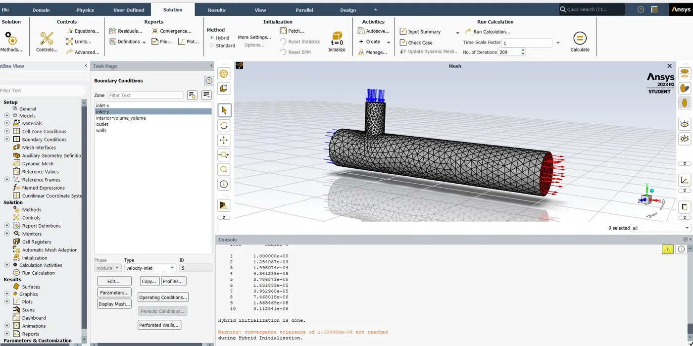
Then next we are ready for run the solver so we re running for 200 iteration.then we got the result.first we started we with scale residuals.

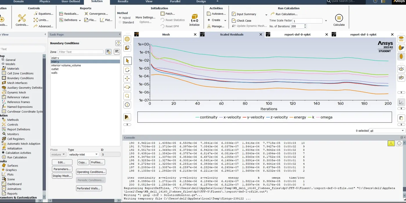
Here the no. of iteration continue the function have been calculated is close to zero. so here we can see that our continuity equation keeping in drcreasing.

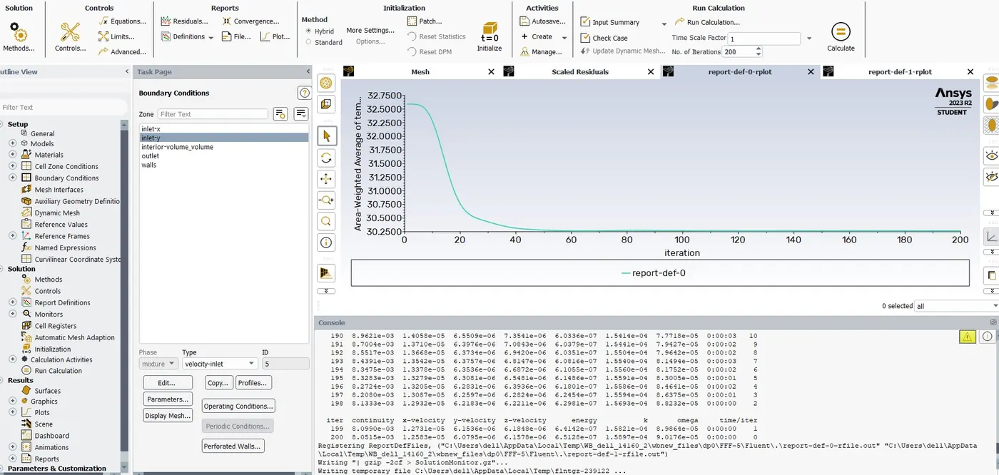
Here we can see that our area weighted temperature is arround 30.280C after that its contineously steady state flow.

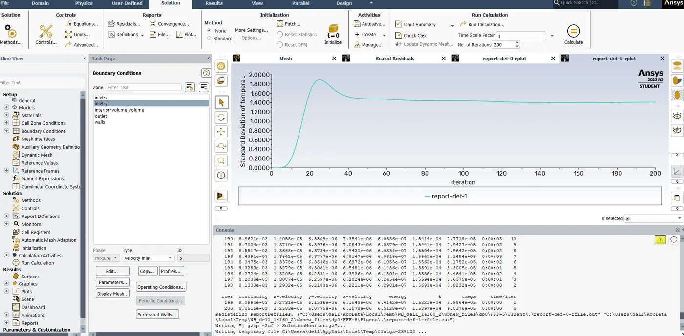
Here we can see that standard deviation of temperature in mixing point is going for highest point then it's going uniformly.

Next we are going for post process the results, so we double click on results after that we can able see our model then we are enable our component we need only our walls, in wall after double clicking then we clicking in rendering then we are applying some transparency. so we need velocity and pressure disturbution. so for that we need to creating a plane xy- plane where the z value is zero.then we got our plane is exactly right in the middle.then we change to that one colour white. after that we can go to plane and then we did colour this one by a variable then we change to temperature then we apply. after we got result then we need bit more changes in range to user specified then we given minmum value of 190C and maximum given as 360C then apply so we seen legend was changed. after that we gone for default legend view then gone to apperance then text parameter to fixed point rotation then its may be 2 decimal places then apply. so we got a good legend view.

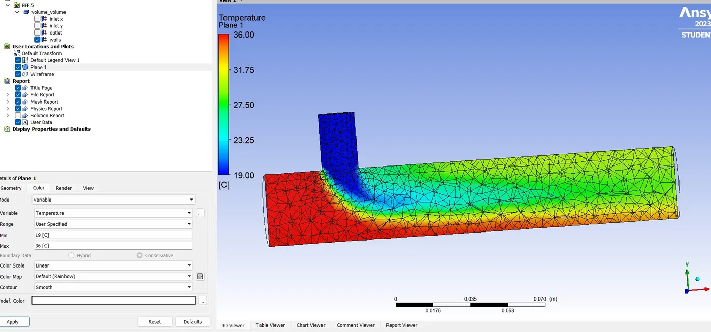
In this first case we used k-omega SST model short mixing tee with a hot inlet velocity 3m/s and momentum ratio 2 taken, so we got good output and good mixing path.so we used both model in first case but we got almost similar output.But, we are good with k-omega SST model. so next case we are using same k-omega SST model.

Next we are going for next one,so here the value model is same only we need to change the momentum. Then directly we are going for setup,after opening of setup we opened the viscous model then we are using here k-omega SST model.Then here maximun value is same. so directly we going for next one that is boundary condiation we are selecting inlet-x , then we seen type is automatically set for velocity-inlet, then we selecting edit then our along inlet face my velocity is 3 m/s.after that incoming hot temperature along the pipe is 360C.then next we are going another velocity inlet that will be our y-axis, where my velocity inlet is 12 m/s and my inlet cold temperature is 190C and we checked our outlet we seen our pressure gauge is zero.

Then next we are going for soving part, in that one we want know what is our oulet temperature, so for that one we clicking in defination then we are interested in computing area weighted average and variable looking for that temperature then we need faces that will be our outlet then we createing report file and report plot and this is done for every iteration then we clicking ok.in this problem we are doing mixing problem, for understand the effectiveness of mixing so we need standard deviation and the variable is temperature and the face is outlet then we can create a another report file and another report plot for that one.once we complete the initial condiation, boundary condiation and material property, then next we are going for initialize the solution.in initialization we are using hybrid initialization then we click the initialize after ten iteration the initialization is done.

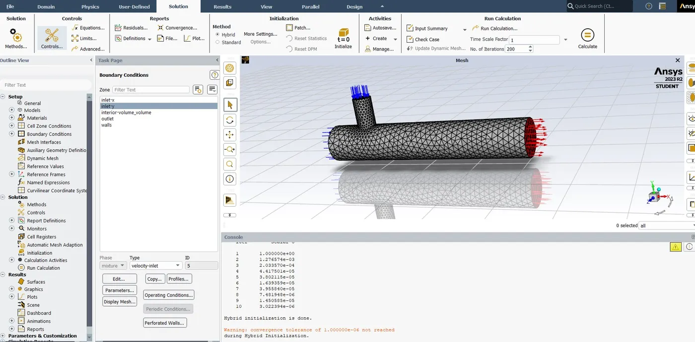
Then next we are ready for run the solver so we re running for 200 iteration.then we got the result.first we started we with scale residuals

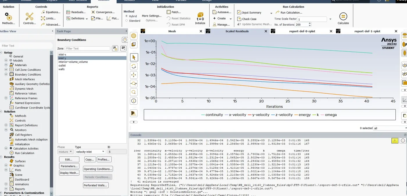
Here the no. of iteration continue the function have been calculated is close to zero. so here we can see that our continuity equation keeping in drcreasing.

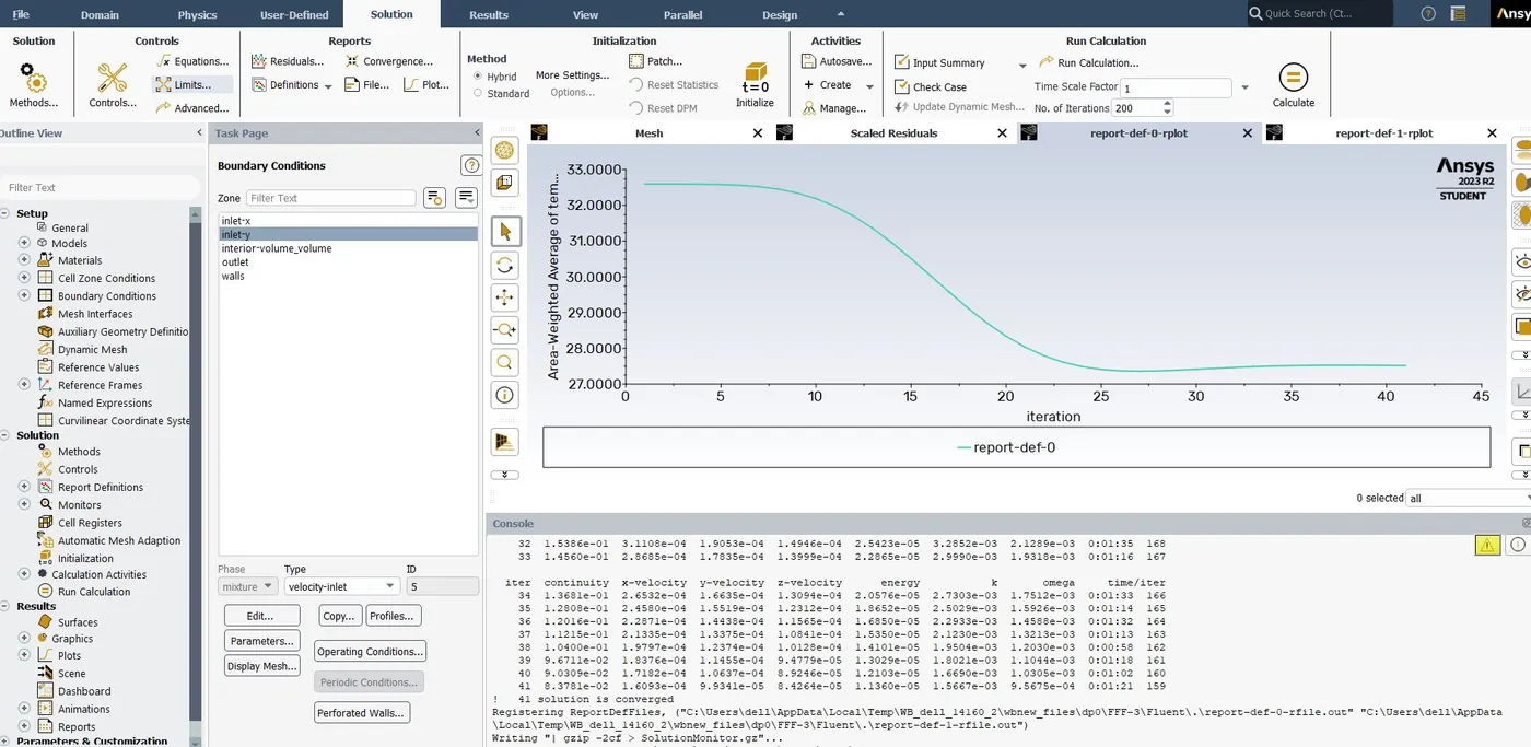
Here we can see that our area weighted temperature is arround 27.800C after that its contineously steady state flow.

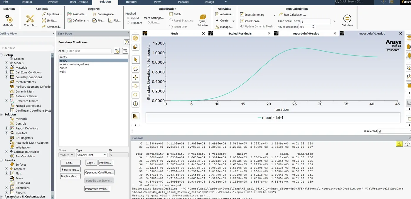
Here we can see that standard deviation of temperature in mixing point is going for highest point then it's going uniformly.

Next we are going for post process the results, so we double click on results after that we can able see our model then we are enable our component we need only our walls, in wall after double clicking then we clicking in rendering then we are applying some transparency. so we need velocity and pressure disturbution. so for that we need to creating a plane xy- plane where the z value is zero.then we got our plane is exactly right in the middle.then we change to that one colour white. after that we can go to plane and then we did colour this one by a variable then we change to temperature then we apply. after we got result then we need bit more changes in range to user specified then we given minmum value of 190C and maximum given as 360C then apply so we seen legend was changed. after that we gone for default legend view then gone to apperance then text parameter to fixed point rotation then its may be 2 decimal places then apply. so we got a good legend view.

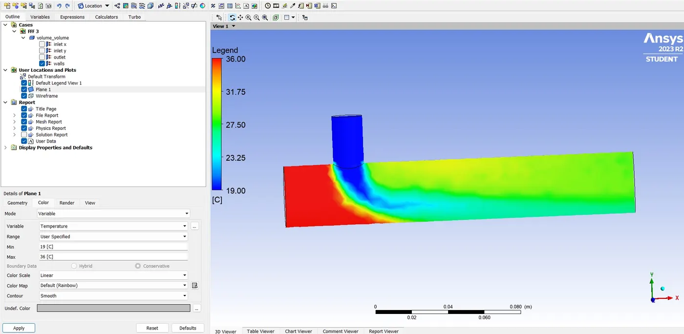
Here we got good output and good mixing path because of velocity inet is more as compare to first one. so we getting a good legend view.

Next we are going for second one case-2, here the long mixing tee with a hot velocity inlet 3 m/s. and momentum ratio of 2,4.In this one we are going with momentum 2.first we opened spaceclaim, in spaceclaim we import the geometry so previously we discussed we started with long mixing tee. after import the geometry we started the geometry clean up. in this long mixing tee we need wall where the heat flux will flow through the body wall. so we seen some surface which one we no need for future activity. then we started to delete those parts. so it will be time consuming process.then we taken option called volume extract, in volume extract we choose edge's after we selected three edges then in down one right mark is there we selected then we seen left corner of tee one more new object added, then we hide the solid component. after that we don't need the solid component in mesh generation process so we did suppress for physics.

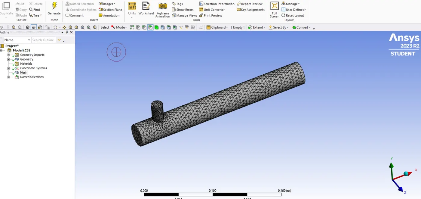
After cad cleanup we started with meshing, in meshing we started with face selection, then we started first selection that will be x-inlet, then second one y-inlet, then 3rd one outlet and last one wall.after selection of face we select the mesh then we started the mesh by default of sizing mesh. after that we got meshing of the body and good element number of count.

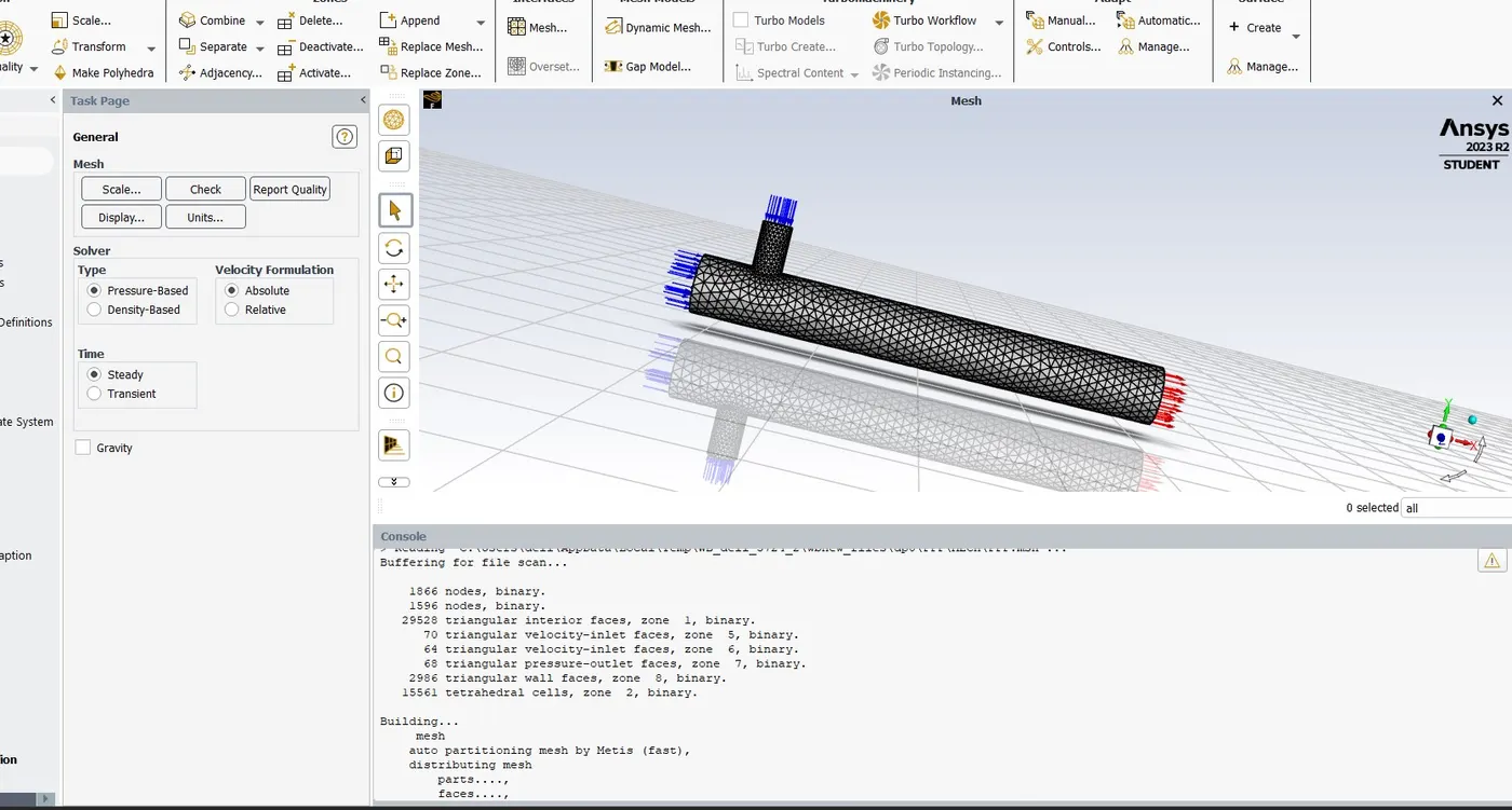
After completing of meshing we started the setup, in setup we selected solver option double precision and parallel simulation and we taken 4 processer then we putted ok. after opening more information printed out automatically.then we gone to the graphics window we seen geometry was there.then we started with mesh checking.then we got our mesh is okay.then we are going to next setting up physics. in this case we taking steady state solver then for small mach number flow we taken pressure-based solver then for velocity formulation absoulte option. then we are interested for solving temperature so we are using energy equation.so in this particular model the flow can be turbulent so that we are using viscous model then we are using k-epsilon model, after that we are using realizable k-epsilon model, then we selected standard wall functions.after we started add material, in add material we seen default one is there air, so we gone through air flow.after that we assign boundary condiation then we are selecting cell zone, in cell zone condiation we are selecting volume then we seen the intenal volume type is fluid.then we going for next one that is boundary then in boundary condiation we are selecting inlet-x , then we seen type is automatically set for velocity-inlet, then we selecting edit then our along inlet face my velocity is 3 m/s.after that incoming hot temperature along the pipe is 360C.then next we are going another velocity inlet that will be our y-axis, where my velocity inlet is 6m/s and my inlet cold temperature is 190C.

Then next we are going for soving part, in that one we want know what is our oulet temperature, so for that one we clicking in defination then we are interested in computing area weighted average and variable looking for that temperature then we need faces that will be our outlet then we createing report file and report plot and this is done for every iteration then we clicking ok.in this problem we are doing mixing problem, for understand the effectiveness of mixing so we need standard deviation and the variable is temperature and the face is outlet then we can create a another report file and another report plot for that one.once we complete the initial condiation, boundary condiation and material property, then next we are going for initialize the solution.in initialization we are using hybrid initialization then we click the initialize after ten iteration the initialization is done.

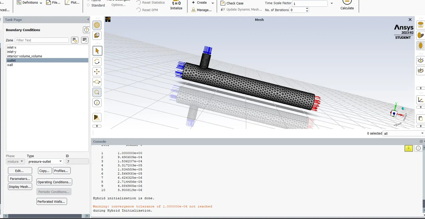
Then next we are ready for run the solver so we re running for 200 iteration.then we got the result.first we started we with scale residuals.

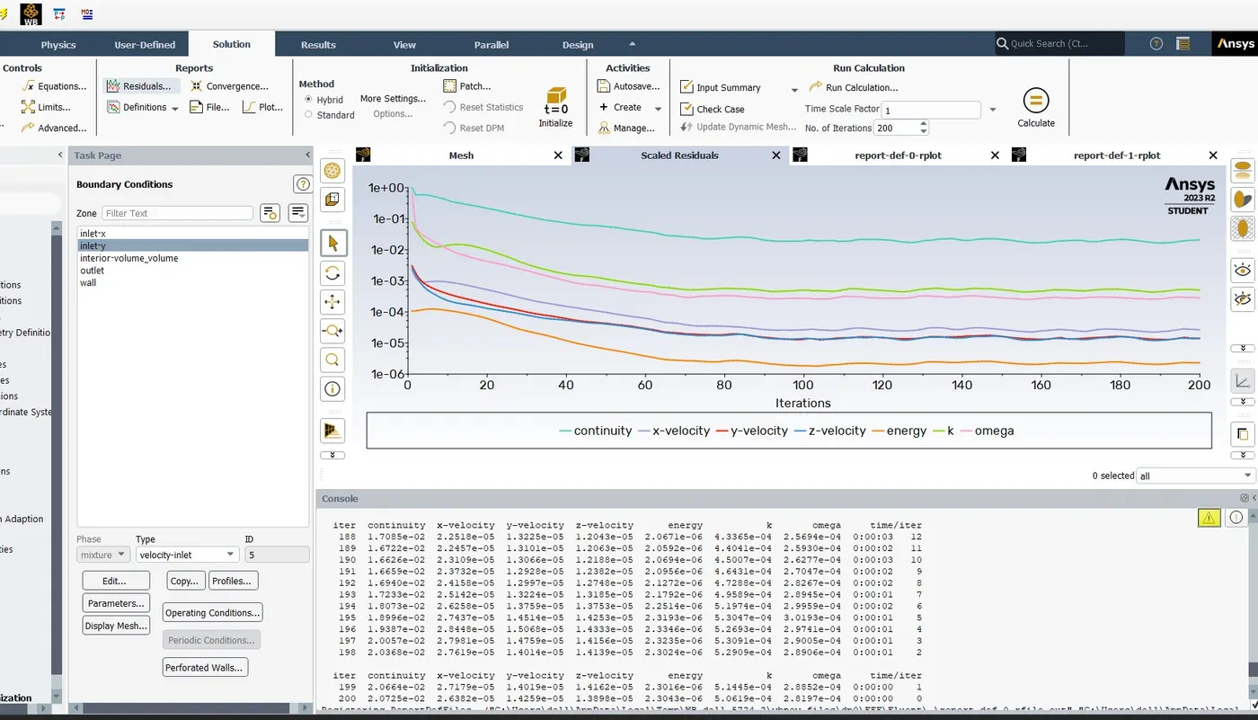
Here the no. of iteration continue the function have been calculated is close to zero. so here we can see that our continuity equation keeping in drcreasing.

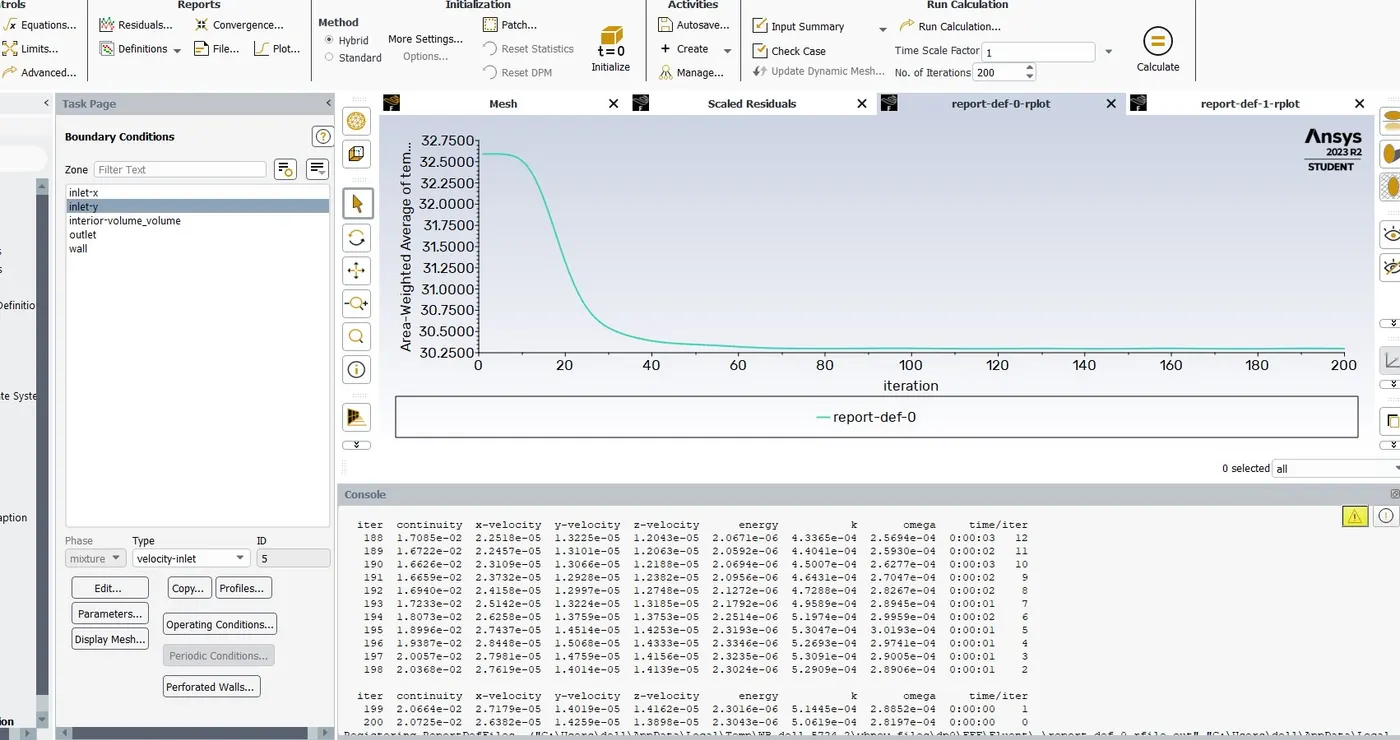
Here we can see that our area weighted temperature is arround 30.300C after that its contineously steady state flow.

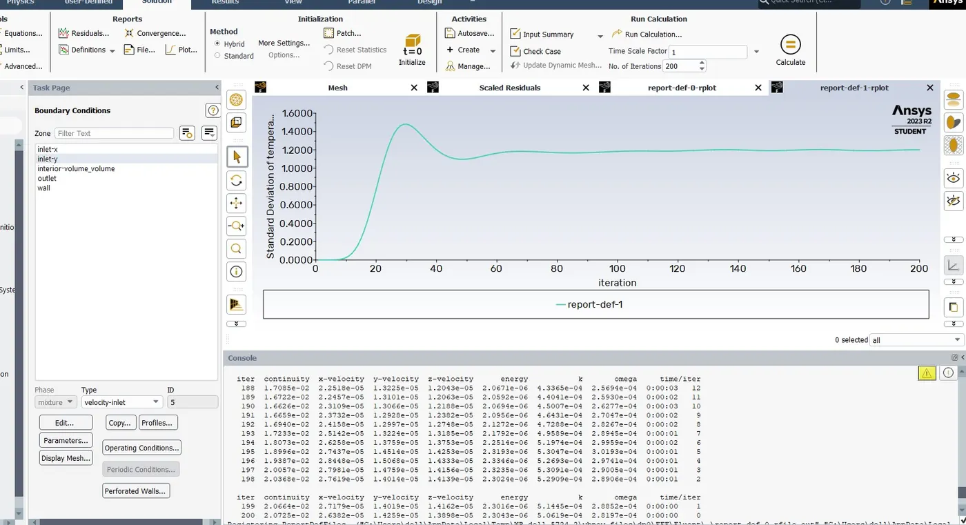
Here we can see that standard deviation of temperature in mixing point is going for highest point then its going uniformly.

Next we are going for post process the results, so we double click on results after that we can able see our model then we are enable our component we need only our walls, in wall after double clicking then we clicking in rendering then we are applying some transparency. so we need velocity and pressure disturbution. so for that we need to creating a plane xy- plane where the z value is zero.then we got our plane is exactly right in the middle.then we change to that one colour white. after that we can go to plane and then we did colour this one by a variable then we change to temperature then we apply. after we got result then we need bit more changes in range to user specified then we given minmum value of 190C and maximum given as 360C then apply so we seen legend was changed. after that we gone for default legend view then gone to apperance then text parameter to fixed point rotation then its may be 2 decimal places then apply. so we got a good legend view.

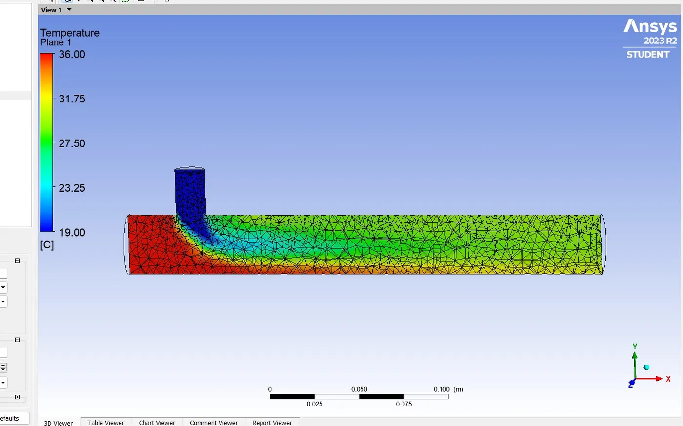
Here we got good output and good mixing path, in this case-2 we got good legend view. next we are going case-2 momentum ratio 4.

Next we are going for next one,so here the value model is same only we need to change the momentum.Then here maximun value is same. so directly we going for next one that is boundary condiation we are selecting inlet-x , then we seen type is automatically set for velocity-inlet, then we selecting edit then our along inlet face my velocity is 3 m/s.after that incoming hot temperature along the pipe is 360C.then next we are going another velocity inlet that will be our y-axis, where my velocity inlet is 12 m/s and my inlet cold temperature is 190C and we checked our outlet we seen our pressure gauge is zero.

Then next we are going for soving part, in that one we want know what is our oulet temperature, so for that one we clicking in defination then we are interested in computing area weighted average and variable looking for that temperature then we need faces that will be our outlet then we createing report file and report plot and this is done for every iteration then we clicking ok.in this problem we are doing mixing problem, for understand the effectiveness of mixing so we need standard deviation and the variable is temperature and the face is outlet then we can create a another report file and another report plot for that one.once we complete the initial condiation, boundary condiation and material property, then next we are going for initialize the solution.in initialization we are using hybrid initialization then we click the initialize after ten iteration the initialization is done.

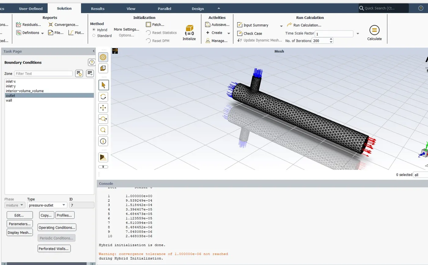
Then next we are ready for run the solver so we re running for 200 iteration.then we got the result.first we started we with scale residuals.

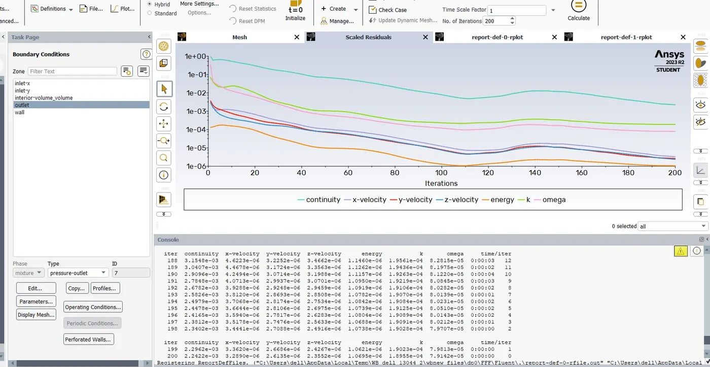
Here the no. of iteration continue the function have been calculated is close to zero. so here we can see that our continuity equation keeping in drcreasing.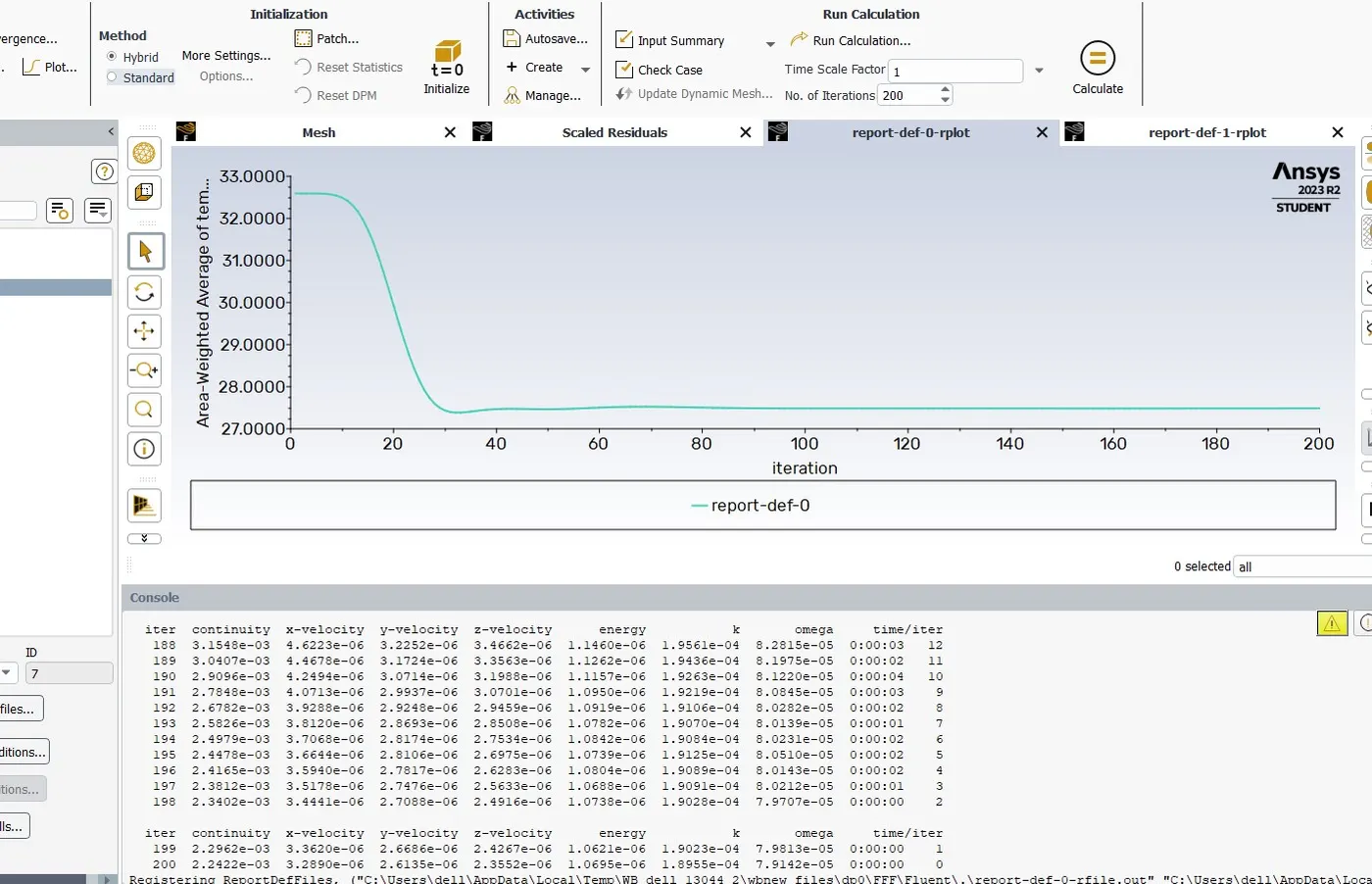

Here we can see that our area weighted temperature is arround 27.400C after that its contineously steady state flow.

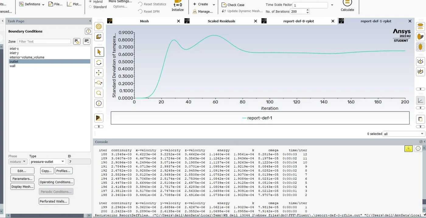
Here we can see that standard deviation of temperature in mixing point is going for highest point then it's going uniformly.

Next we are going for post process the results, so we double click on results after that we can able see our model then we are enable our component we need only our walls, in wall after double clicking then we clicking in rendering then we are applying some transparency. so we need velocity and pressure disturbution. so for that we need to creating a plane xy- plane where the z value is zero.then we got our plane is exactly right in the middle.then we change to that one colour white. after that we can go to plane and then we did colour this one by a variable then we change to temperature then we apply. after we got result then we need bit more changes in range to user specified then we given minmum value of 190C and maximum given as 360C then apply so we seen legend was changed. after that we gone for default legend view then gone to apperance then text parameter to fixed point rotation then its may be 2 decimal places then apply. so we got a good legend view.

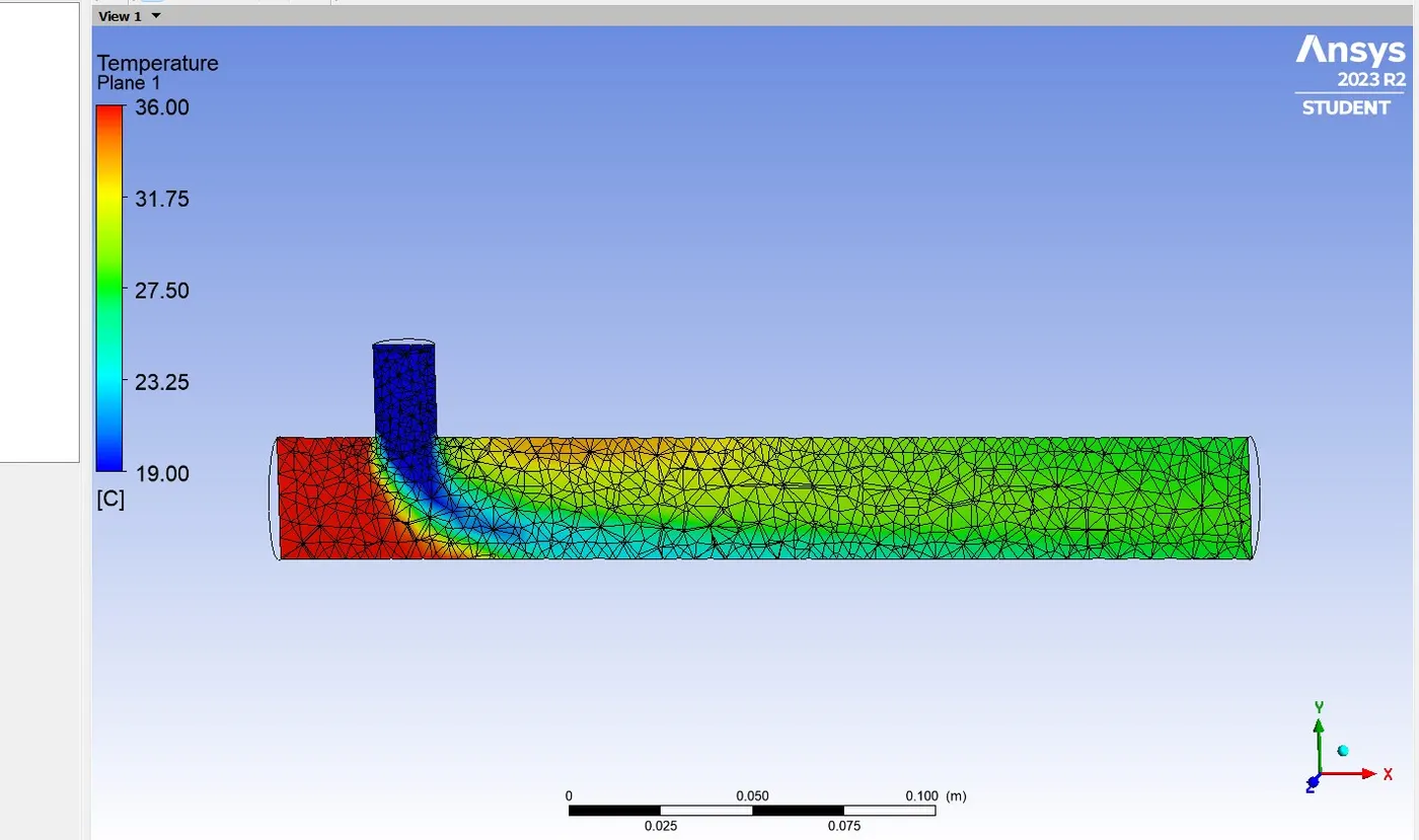
Here we got good output and good mixing path because of velocity inet is more as compare to first one and also we getting a good legend view.

1)Here the cell count in first case is 12613.

Then second case cell count is 15561.

2) In first case Average outlet temperature is 30.290C.

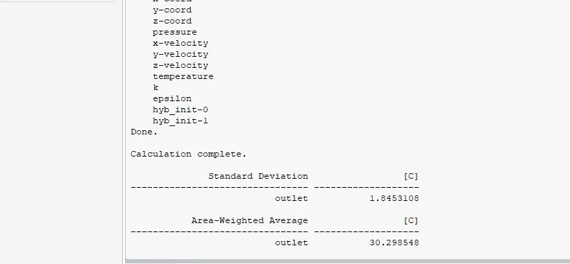
Then second case Average outlet temperature is 27.850C.

Due to different inlet velocity and short & long mixing tee so outlet temperature is vary.

3) Both case Number of iterations for convergence, we taken 200 iterations.

Next we are going for expected results.

1) Velocity and temperature contour plots on the cut planes along and across the pipe for first case1, For Short mixing tee.

So first we started with Velocity contour plots on the cut planes along and across the pipe for first case, in first case 2 momentum is there, so first we taken momentum 2, for that one first we started to create the plane across the pipe, then we insert the plane one by one and we taken yz direction. after completion of inserting plane we started for calculate veloctiy.then we gone for every plane and we clicked in color we changed variable to velocity then we got the result.

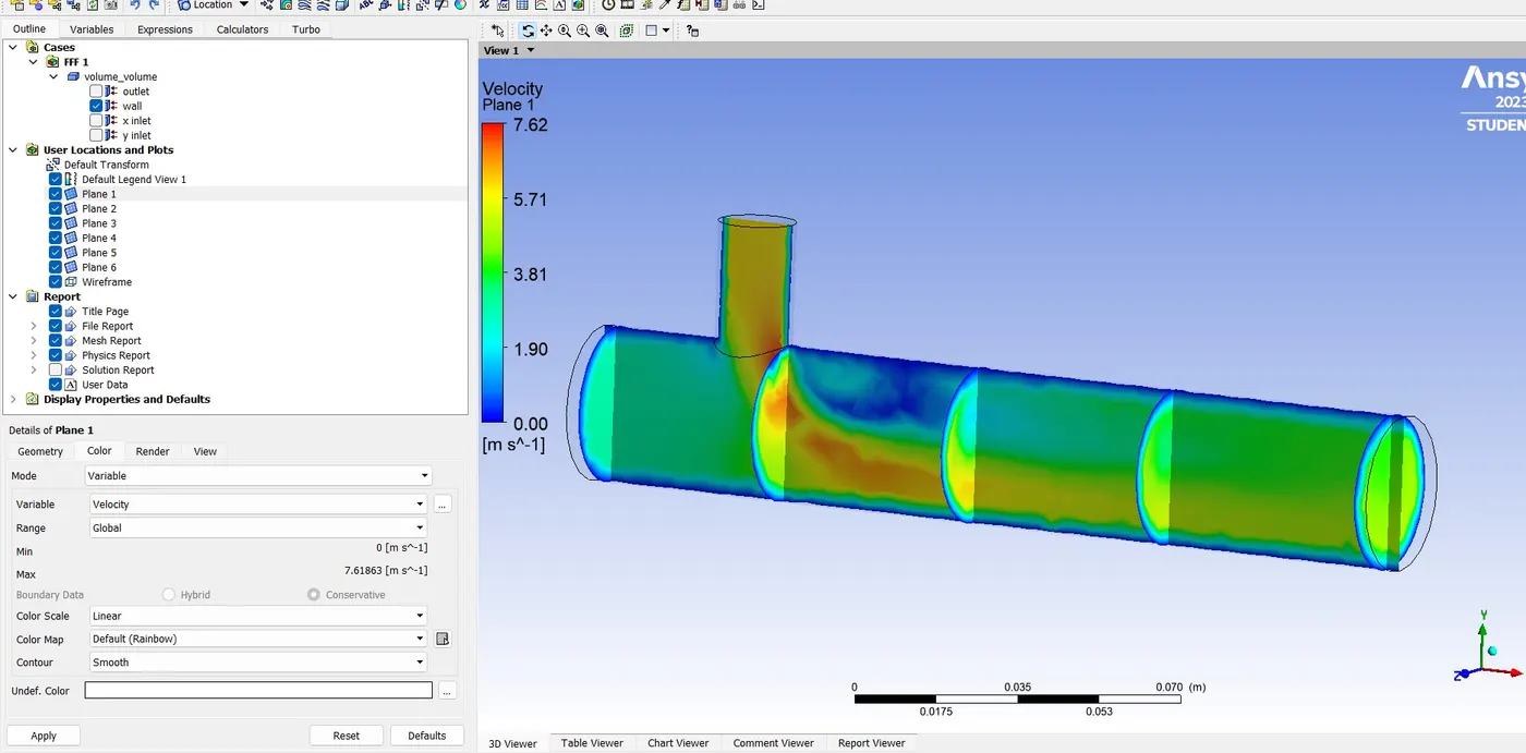
Then next we are going for temperature contour plots on the cut planes along and across the pipe.then, we started for calculate the temperature, for that one we gone for every plane and we clicked in color we changed variable to temperature then we got the result.

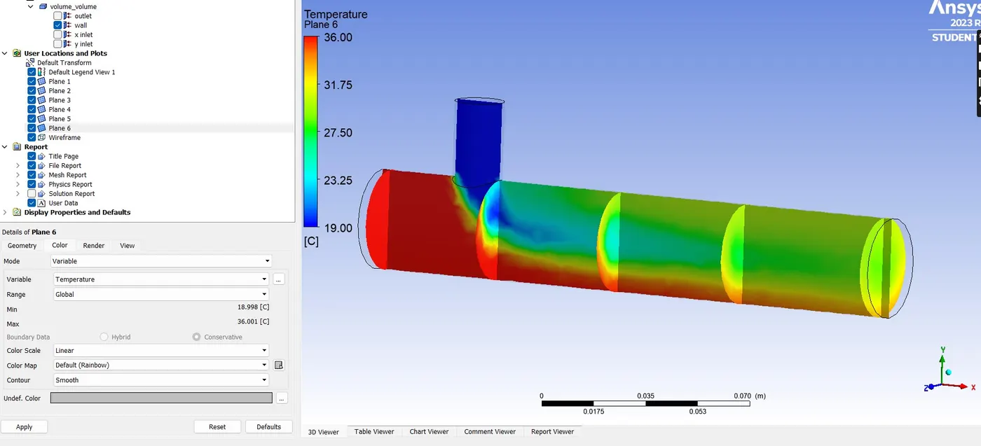
2) Velocity and temperature line plots along and across the length of the pipe for case 1. then we gone for insert line and we created the both line both direction.

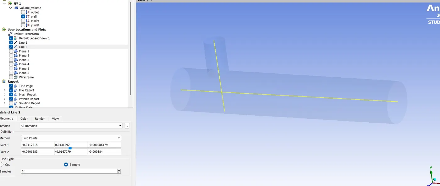
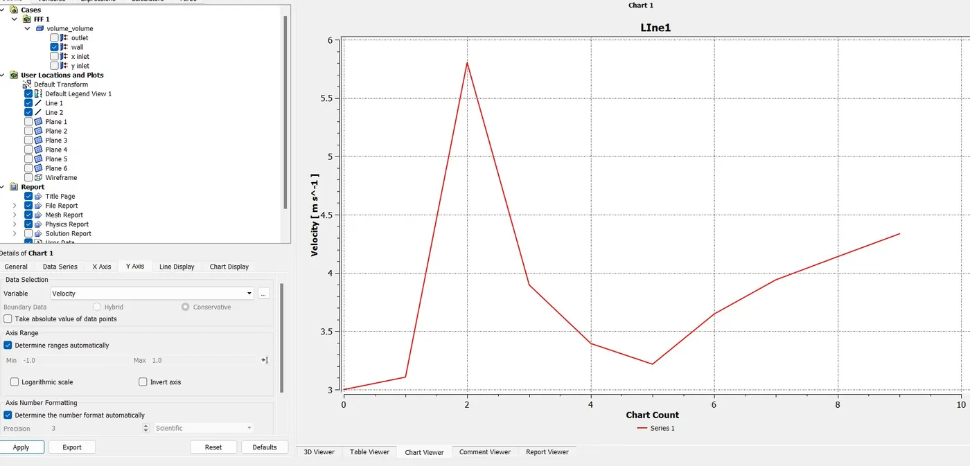
Next we are going for Velocity line plots along the length of the pipe. so for that one we insert a chart, then in chart we gone for data series in that one we taken series 1 and then we location we taken line 1 then we taken x-axis, in x-axis we taken the varible chart count , then in y-axis we taken variable velocity. After that we did apply we got result.

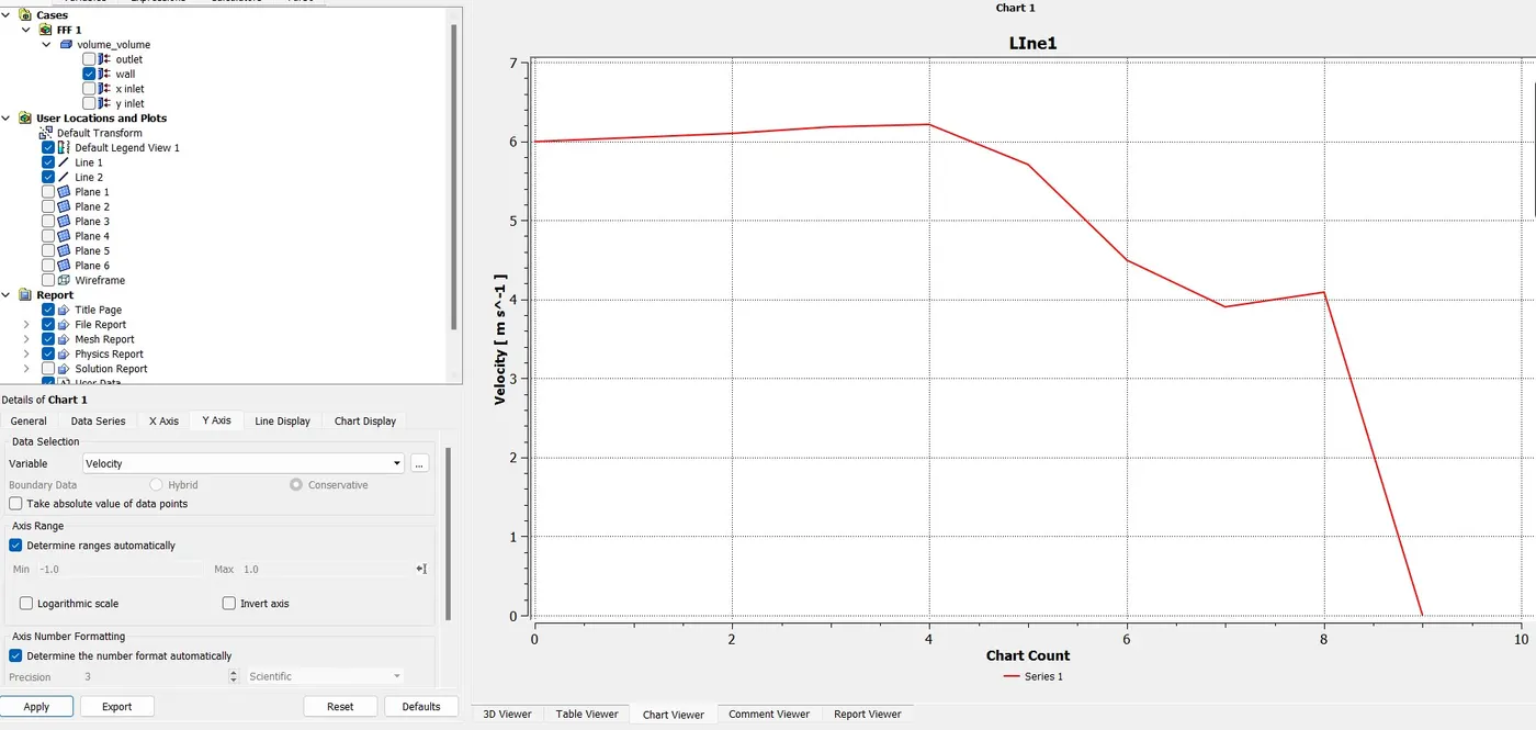
Then next one we are going for Velocity line plots across the length of the pipe. in this one in chart we gone for data series in that one we taken series 1 and then we location we taken line 2 then we taken x-axis, in x-axis we taken the varible chart count , then in y-axis we taken variable velocity. After that we did apply we got result.

Then next one we are going for temperature line plots along the length of the pipe. in this one in chart we gone for data series in that one we taken series 1 and then we location we taken line 1 then we taken x-axis, in x-axis we taken the varible chart count , then in y-axis we taken variable temperature. After that we did apply we got result.

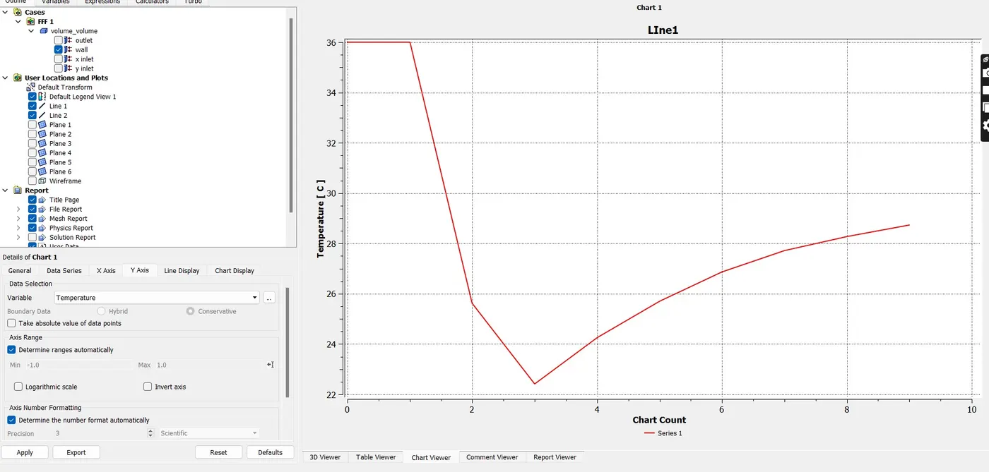
Then next one we are going for temperature line plots across the length of the pipe. in this one in chart we gone for data series in that one we taken series 1 and then we location we taken line 2 then we taken x-axis, in x-axis we taken the varible chart count , then in y-axis we taken variable temperature. After that we did apply we got result.

Next we are going for

1) Velocity and temperature contour plots on the cut planes along and across the pipe for first case1 momentum 4.

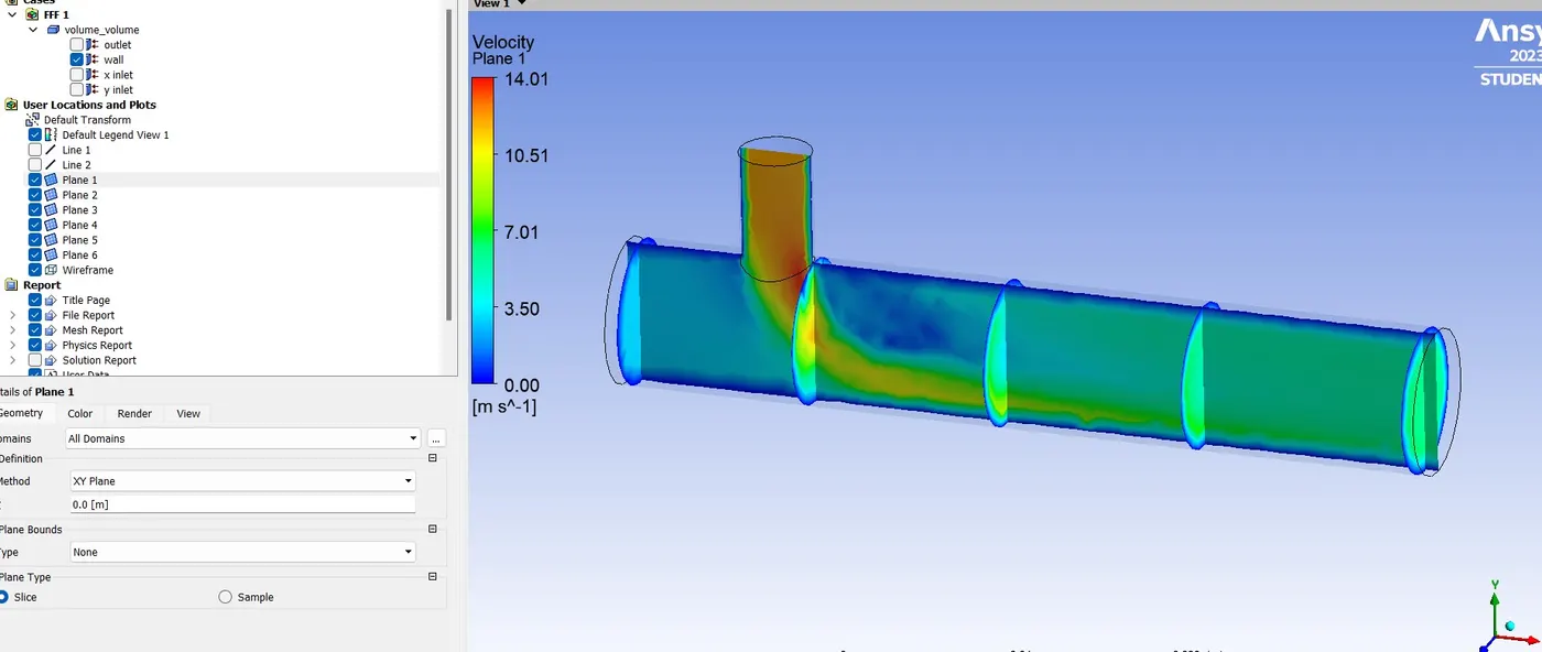
So here we started with Velocity contour plots on the cut planes along and across the pipe for first case,In first case we are taking momentum 4, for changing momentum we went to setup then we change the cold inlet velocity 12 m/s and temperature 190C. After that we run the simulation then we got result then again we are going for post processing, then we checked all our data is there, then we started for calculate veloctiy, then we gone for every plane and we clicked in color we changed variable to velocity then we got the result.

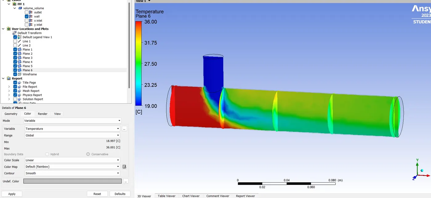
Then next we are going for temperature contour plots on the cut planes along and across the pipe.then, we started for calculate the temperature, for that one we gone for every plane and we clicked in color we changed variable to temperature then we got the result.

2) Velocity and temperature line plots along and across the length of the pipe for case 1 momentum 4.

Next we are going for Velocity line plots along the length of the pipe. Then we gone for data series in that one we taken series 1 and then we location we taken line 1 then we taken x-axis, in x-axis we taken the varible chart count , then in y-axis we taken variable velocity. After that we did apply we got result.

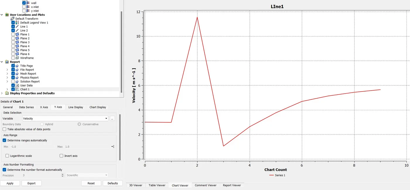
Then next one we are going for Velocity line plots across the length of the pipe. in this one in chart we gone for data series in that one we taken series 1 and then we location we taken line 2 then we taken x-axis, in x-axis we taken the varible chart count , then in y-axis we taken variable velocity. After that we did apply we got result.

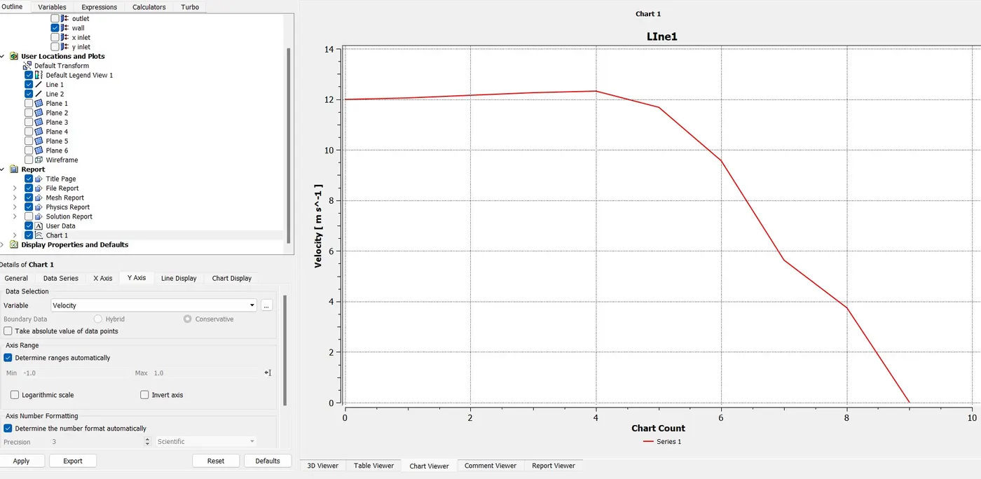
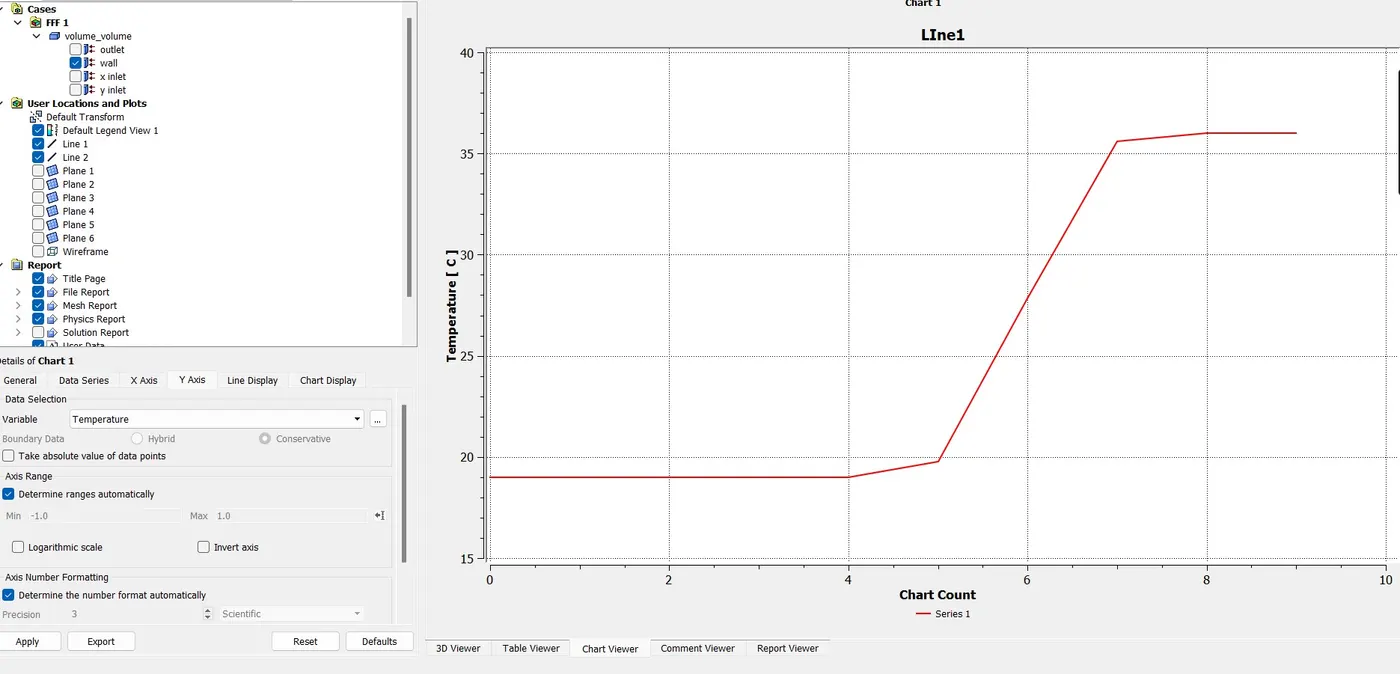
Then next one we are going for temperature line plots along the length of the pipe. in this one in chart we gone for data series in that one we taken series 1 and then we location we taken line 1 then we taken x-axis, in x-axis we taken the varible chart count , then in y-axis we taken variable temperature. After that we did apply we got result.

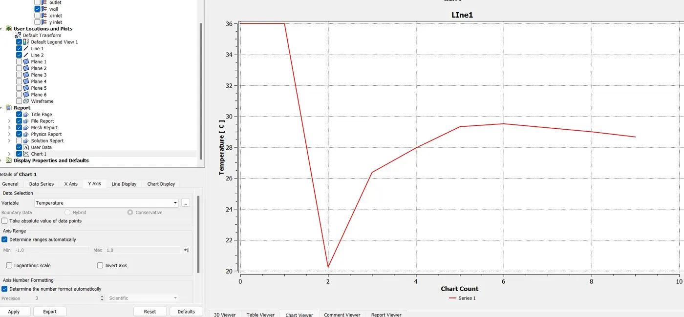
Then next one we are going for temperature line plots across the length of the pipe. in this one in chart we gone for data series in that one we taken series 1 and then we location we taken line 2 then we taken x-axis, in x-axis we taken the varible chart count , then in y-axis we taken variable temperature. After that we did apply we got result.

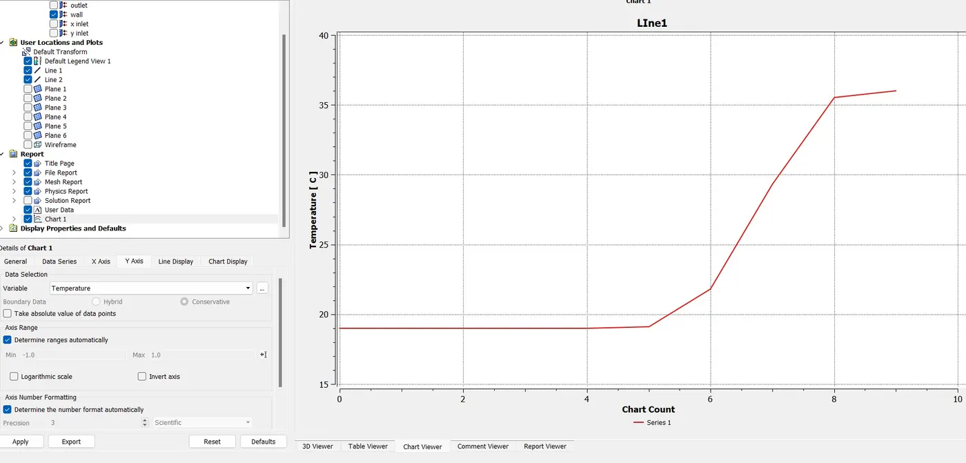
1) Velocity and temperature contour plots on the cut planes along and across the pipe for first case 2 and momentum 2

.For long mixing tee.

So first we started with Velocity contour plots on the cut planes along and across the pipe for first case, In Second case momentum 2 is there, so first we taken momentum 2, for that one first we started to create the plane across the pipe, then we insert the plane one by one and we taken yz direction. after completion of inserting plane we started for calculate veloctiy.then we gone for every plane and we clicked in color we changed variable to velocity then we got the result.

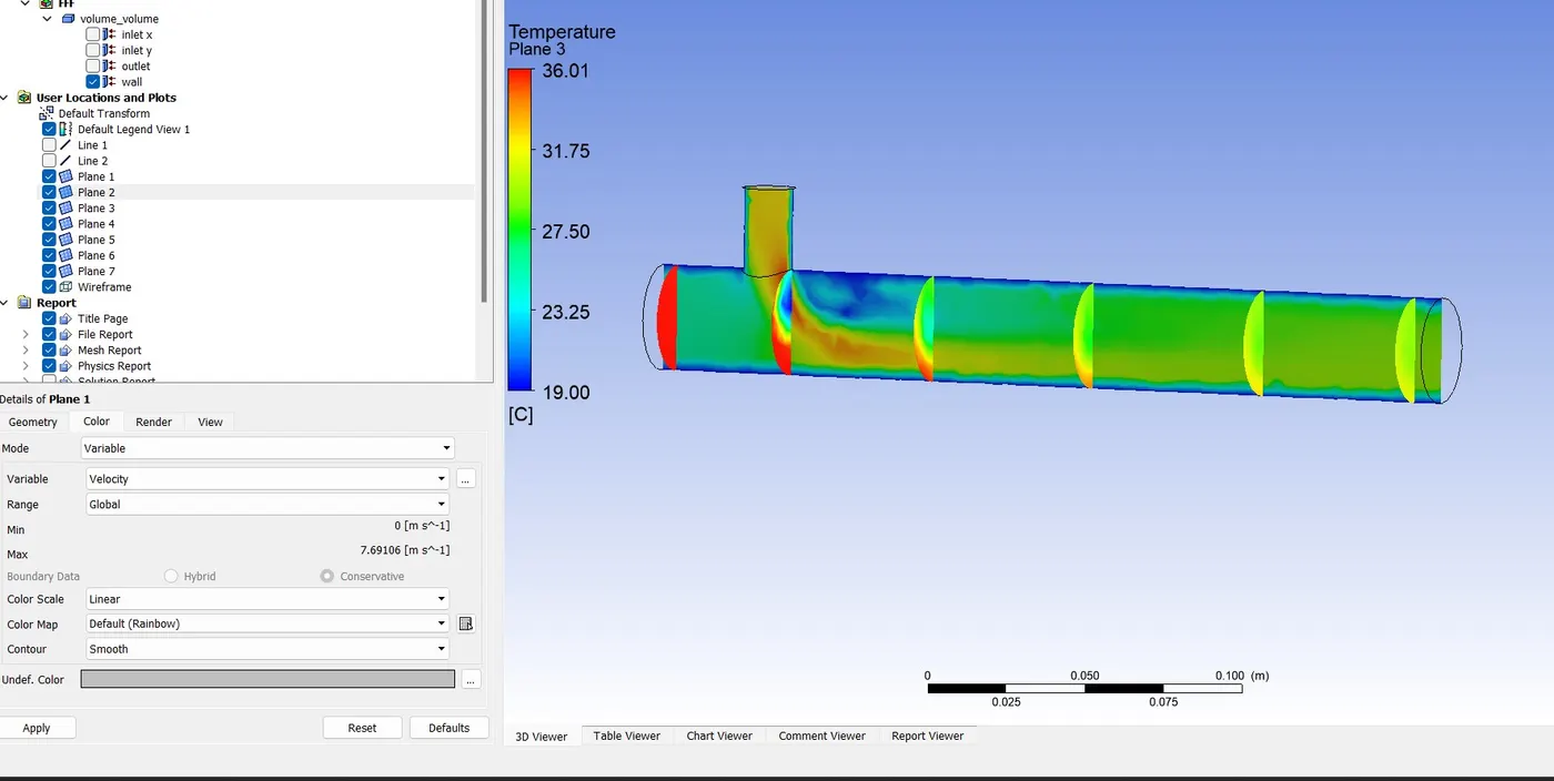
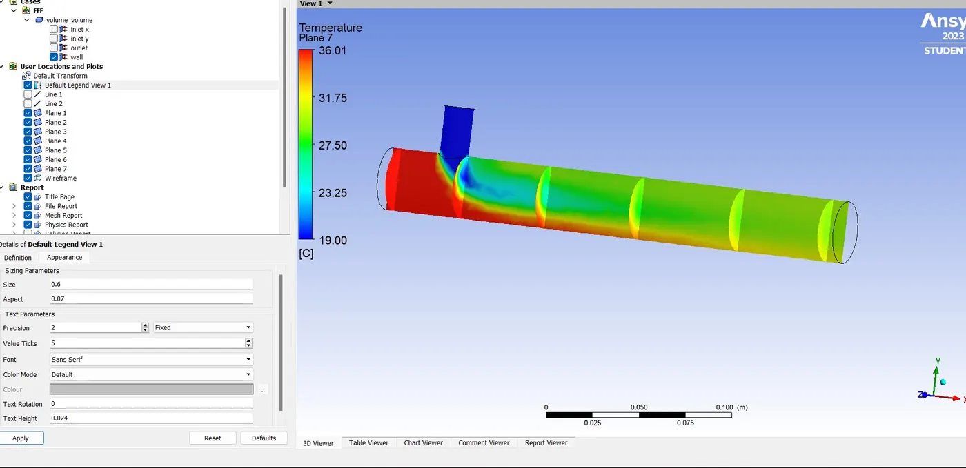
Then next we are going for temperature contour plots on the cut planes along and across the pipe.then, we started for calculate the temperature, for that one we gone for every plane and we clicked in color we changed variable to temperature then we got the result.

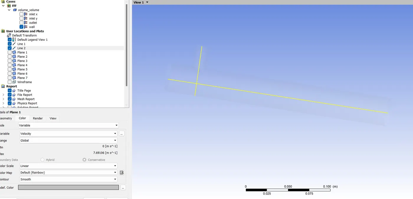
2) Velocity and temperature line plots along and across the length of the pipe for case 2. then we gone for insert line and we created the both line both direction.

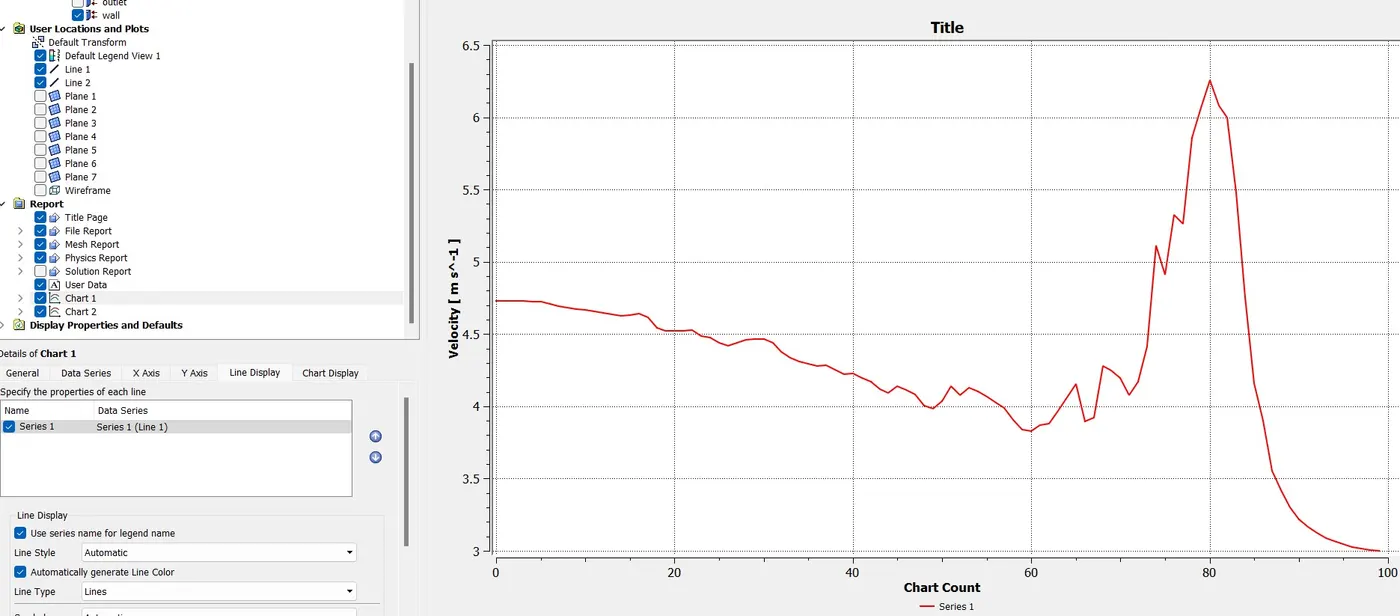
Next we are going for Velocity line plots along the length of the pipe. so for that one we insert a chart, then in chart we gone for data series in that one we taken series 1 and then we location we taken line 1 then we taken x-axis, in x-axis we taken the varible chart count , then in y-axis we taken variable velocity. After that we did apply we got result.

Then next one we are going for Velocity line plots across the length of the pipe. in this one in chart we gone for data series in that one we taken series 1 and then we location we taken line 2 then we taken x-axis, in x-axis we taken the varible chart count , then in y-axis we taken variable velocity. After that we did apply we got result.

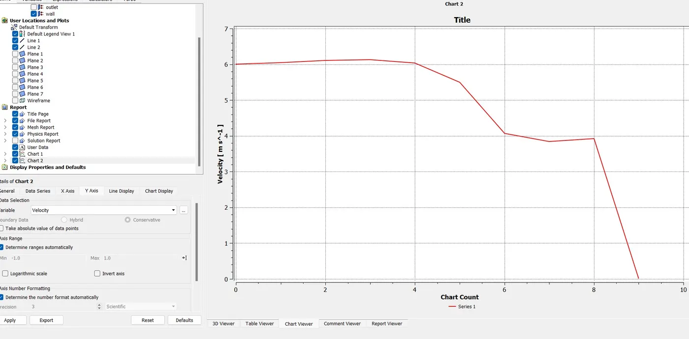
Then next one we are going for temperature line plots along the length of the pipe. in this one in chart we gone for data series in that one we taken series 1 and then we location we taken line 1 then we taken x-axis, in x-axis we taken the varible chart count , then in y-axis we taken variable temperature. After that we did apply we got result.

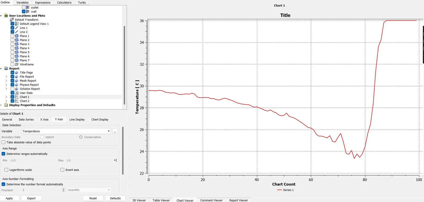
Then next one we are going for temperature line plots across the length of the pipe. in this one in chart we gone for data series in that one we taken series 1 and then we location we taken line 2 then we taken x-axis, in x-axis we taken the varible chart count , then in y-axis we taken variable temperature. After that we did apply we got result.

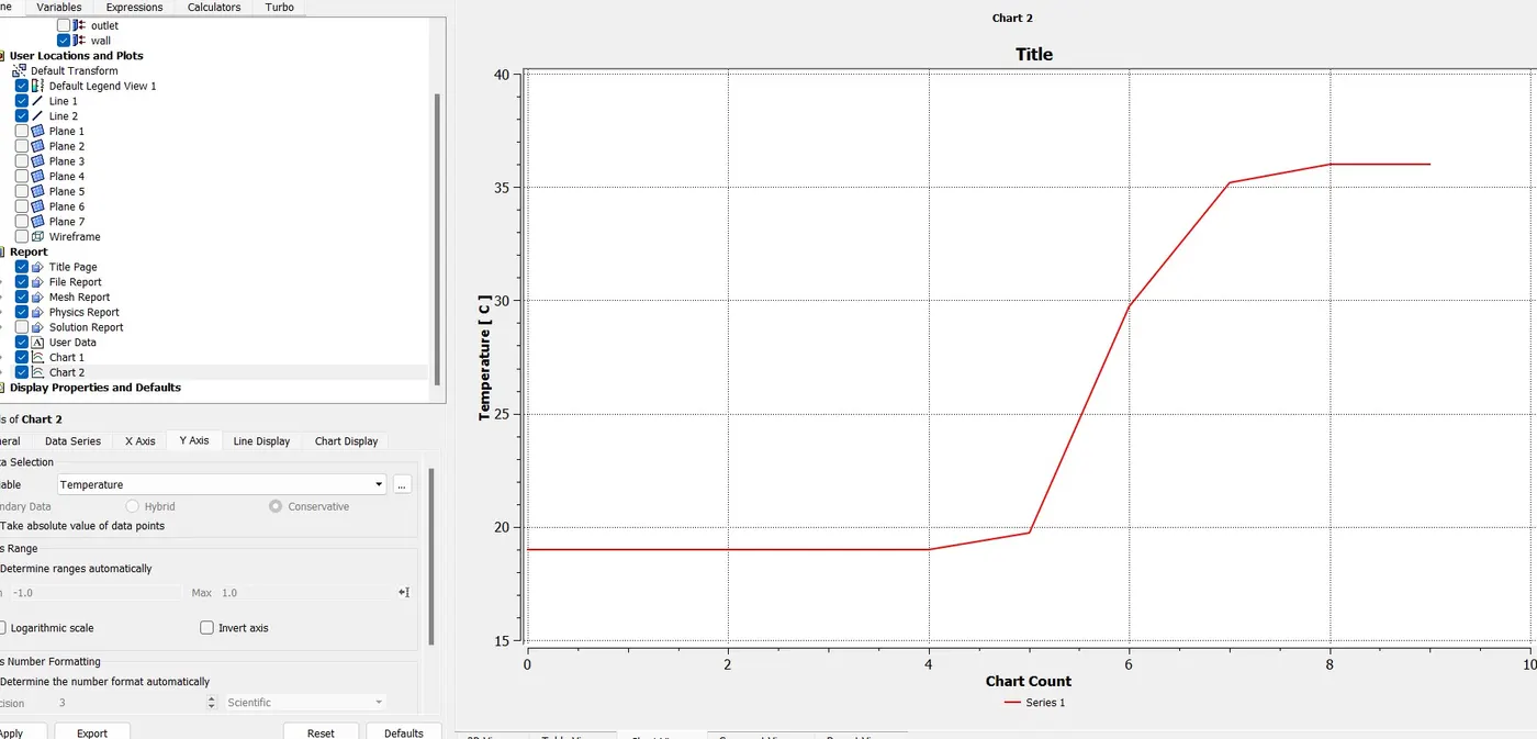
Next we are going for

1) Velocity and temperature contour plots on the cut planes along and across the pipe for first case1 momentum 4.

So here we started with Velocity contour plots on the cut planes along and across the pipe for first case,In first case we are taking momentum 4, for changing momentum we went to setup then we change the cold inlet velocity 12 m/s and temperature 190C. After that we run the simulation then we got result then again we are going for post processing, then we checked all our data is there, then we started for calculate veloctiy, then we gone for every plane and we clicked in color we changed variable to velocity then we got the result.

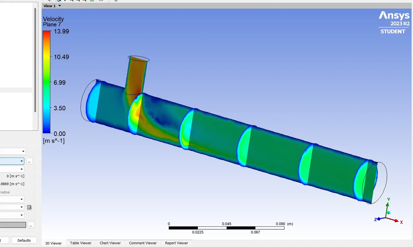
Then next we are going for temperature contour plots on the cut planes along and across the pipe.then, we started for calculate the temperature, for that one we gone for every plane and we clicked in color we changed variable to temperature then we got the result.

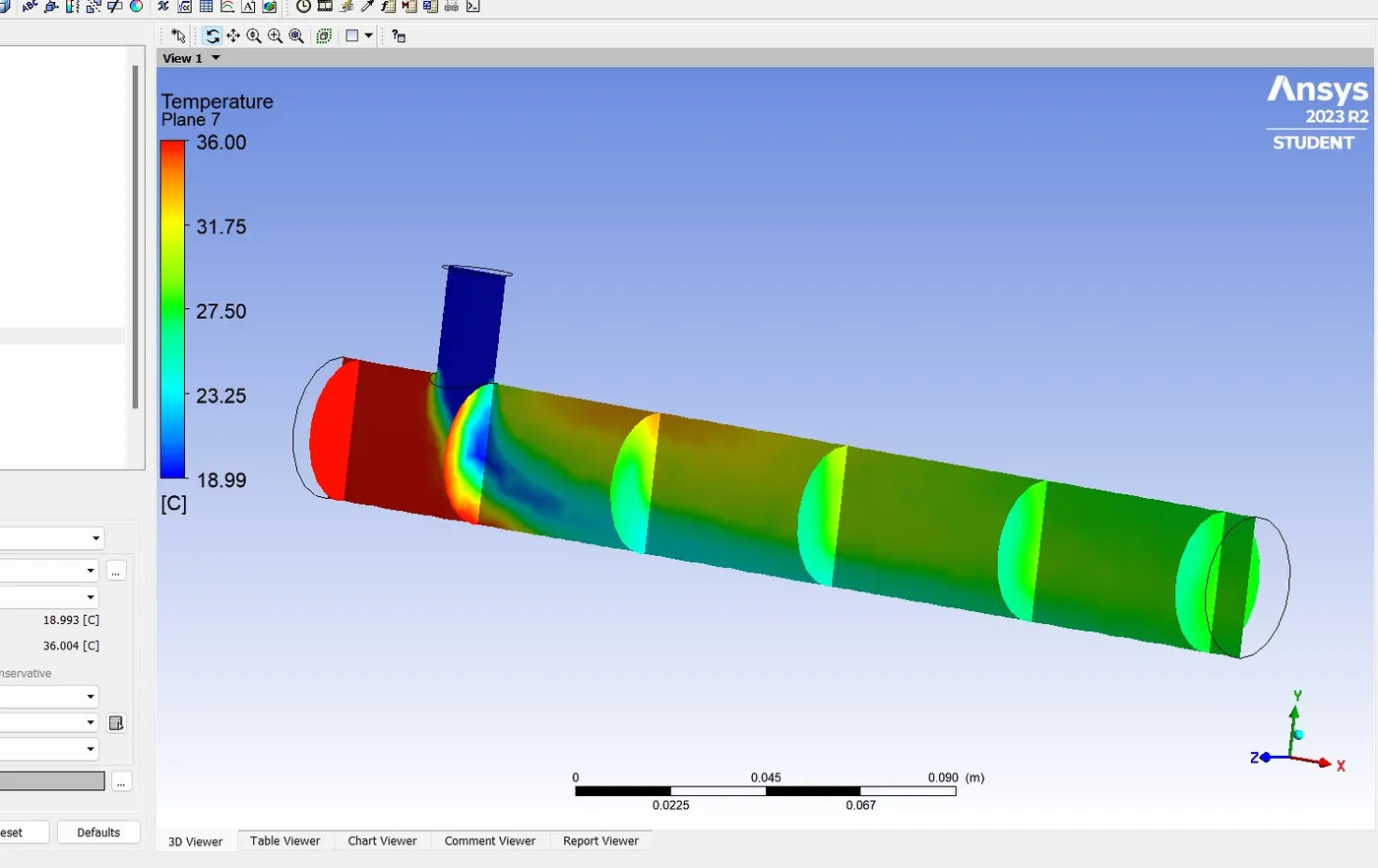
2) Velocity and temperature line plots along and across the length of the pipe for case 1 momentum 4.

Next we are going for Velocity line plots along the length of the pipe. Then we gone for data series in that one we taken series 1 and then we location we taken line 1 then we taken x-axis, in x-axis we taken the varible chart count , then in y-axis we taken variable velocity. After that we did apply we got result.

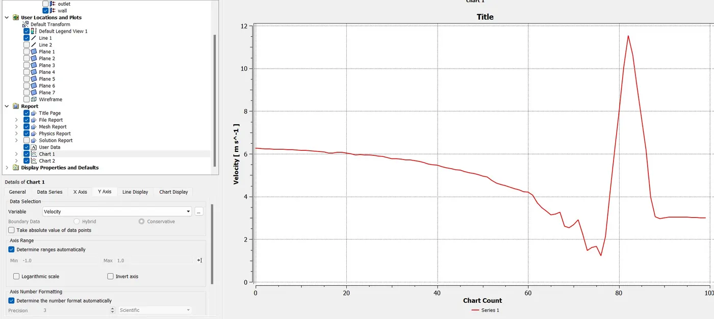
Then next one we are going for Velocity line plots across the length of the pipe. in this one in chart we gone for data series in that one we taken series 1 and then we location we taken line 2 then we taken x-axis, in x-axis we taken the varible chart count , then in y-axis we taken variable velocity. After that we did apply we got result.

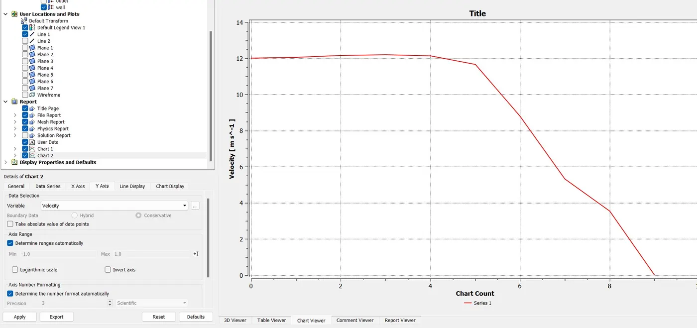
Then next one we are going for temperature line plots along the length of the pipe. in this one in chart we gone for data series in that one we taken series 1 and then we location we taken line 1 then we taken x-axis, in x-axis we taken the varible chart count , then in y-axis we taken variable temperature. After that we did apply we got result.

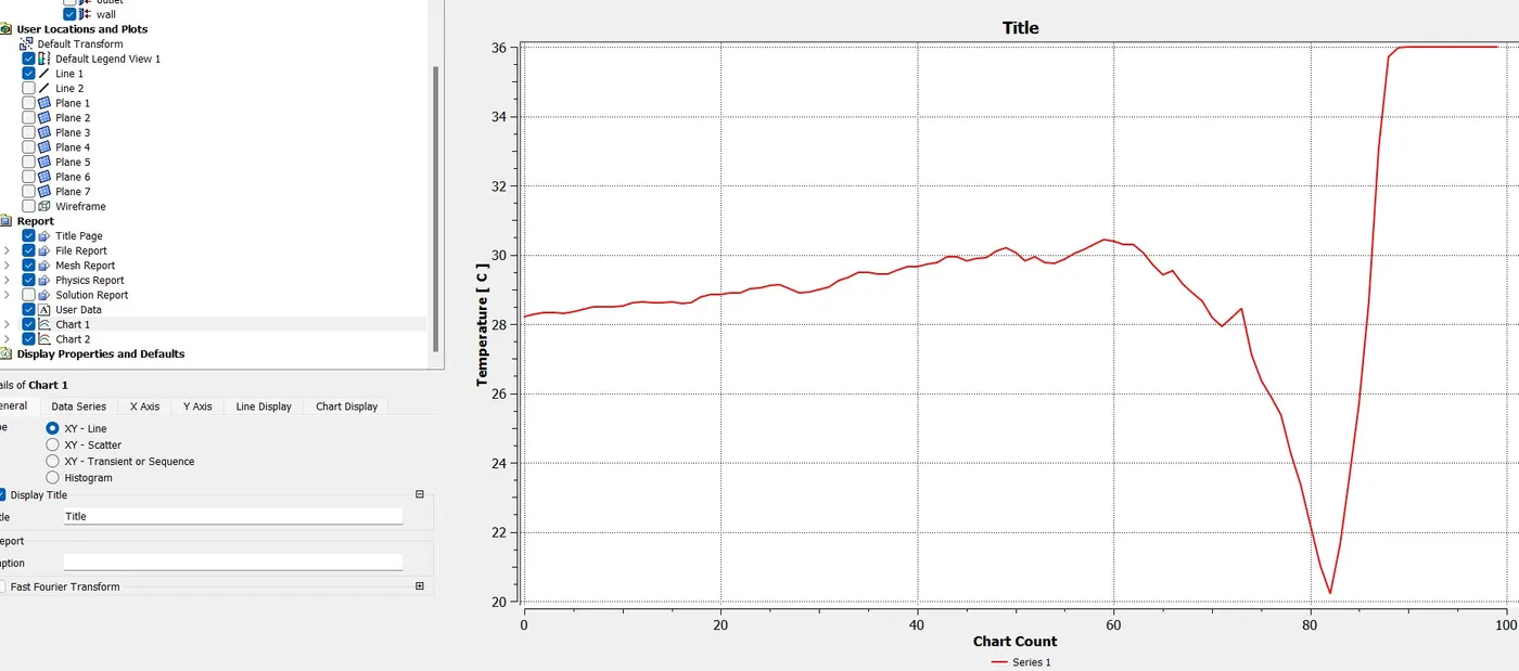
Then next one we are going for temperature line plots across the length of the pipe. in this one in chart we gone for data series in that one we taken series 1 and then we location we taken line 2 then we taken x-axis, in x-axis we taken the varible chart count , then in y-axis we taken variable temperature. After that we did apply we got result.

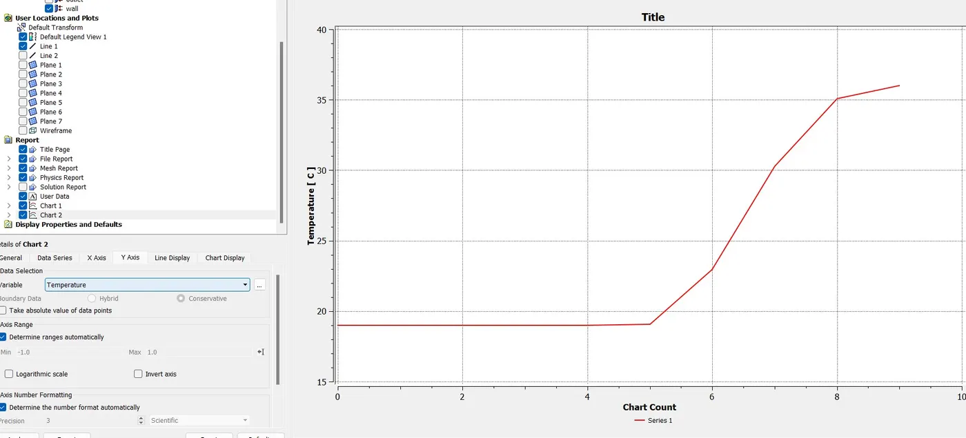
3) Next we are going for Perform Mesh independent study for any one case.

So first we started with import the geometry then did geometry claen up, after that we did suppress for physics.In case 1 there are two momentum ratio is there, so first we started with momentum 2.after cad cleanup we started with meshing, in meshing we started with face selection, then we started first selection that will be x-inlet, then second one y-inlet, then 3rd one outlet and last one wall.after selection of face we select the mesh then we started the mesh by sizing mesh. in sizing we changed the element size.then we got 106587 elements.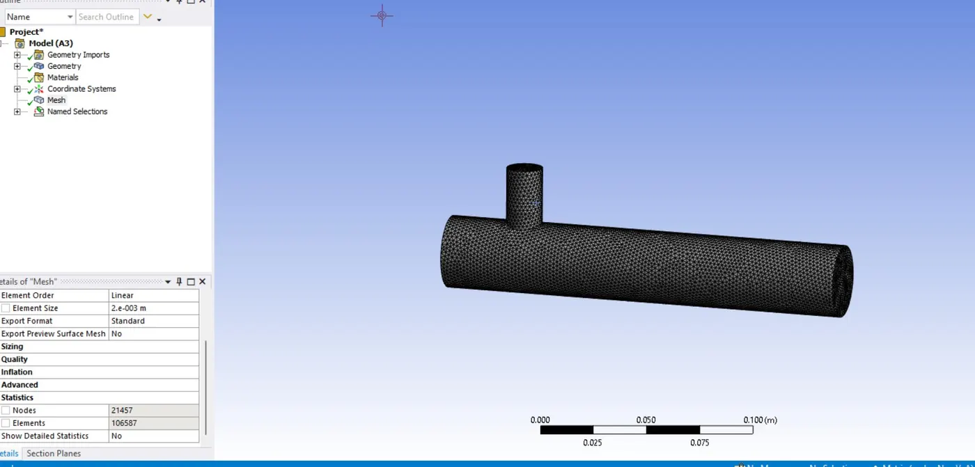

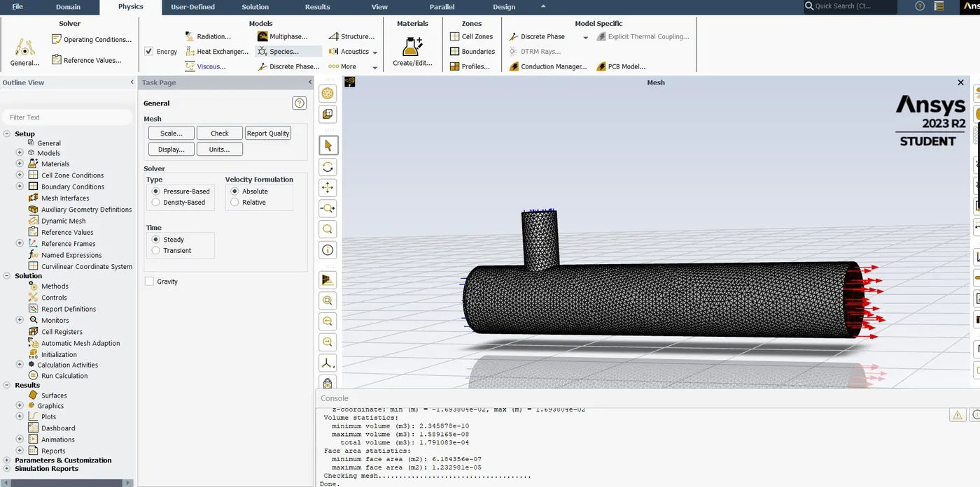
After completing of meshing we started the setup, in setup we selected solver option double precision and parallel simulation and we taken 4 processer then we putted ok. after opening more information printed out automatically.then we gone to the graphics window we seen geometry was there.then we started with mesh checking.then we got our mesh is okay.then we are going to next setting up physics. in this case we taking steady state solver then for small mach number flow we taken pressure-based solver then for velocity formulation absoulte option. then we are interested for solving temperature so we are using energy equation.so in this particular model the flow can be turbulent so that we are using viscous model then we are using k-omega SST. after we started add material, in add material we seen default one is there air, so we gone through air flow.after that we assign boundary condiation then we are selecting cell zone, in cell zone condiation we are selecting volume then we seen the intenal volume type is fluid.then we going for next one that is boundary then in boundary condiation we are selecting inlet-x , then we seen type is automatically set for velocity-inlet, then we selecting edit then our along inlet face my velocity is 3 m/s.after that incoming hot temperature along the pipe is 360C.then next we are going another velocity inlet that will be our y-axis, where my velocity inlet is 6m/s and my inlet cold temperature is 190C.

Then next we are going for soving part, in that one we want know what is our oulet temperature, so for that one we clicking in defination then we are interested in computing area weighted average and variable looking for that temperature then we need faces that will be our outlet then we createing report file and report plot and this is done for every iteration then we clicking ok.in this problem we are doing mixing problem, for understand the effectiveness of mixing so we need standard deviation and the variable is temperature and the face is outlet then we can create a another report file and another report plot for that one.once we complete the initial condiation, boundary condiation and material property, then next we are going for initialize the solution.in initialization we are using hybrid initialization then we click the initialize after ten iteration the initialization is done.

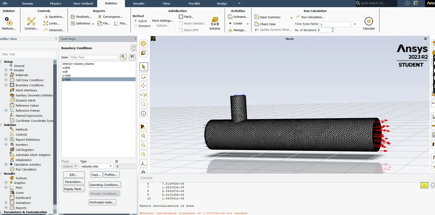
Then next we are ready for run the solver so we re running for 200 iteration.then we got the result.first we started we with scale residuals.

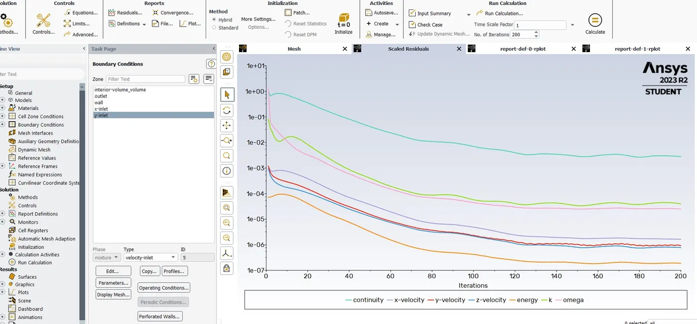
Here the no. of iteration continue the function have been calculated is close to zero. so here we can see that our continuity equation keeping in drcreasing.

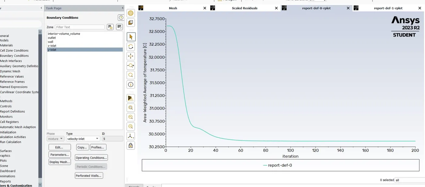
Here we can see that our area weighted average temperature is arround 30.400C after that its contineously steady state flow.

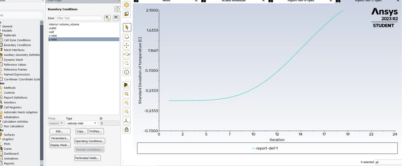
Here we can see that our area weighted temperature is arround 27.400C after that its contineously steady state flow.

4) Here the effect of length and momentum ratio, we checked both case when the momentum is more then we are getting mixing path is smoth.when momentum ratio is less,mixing path deflection is more. so we got the good output smoth mixing path, when the momentum is more.