Week 1- Mixing Tee

Aim: To set up steady-state simulations to compare the mixing effectiveness when hot inlet temperature is 36⁰C & the Cold inlet is at 19⁰C for the two versions of the mixing tee (one of them is longer than the other), for the below two cases:

1. Case 1
• Short mixing tee with a hot inlet velocity of 3m/s.
• Momentum ratio of 2, 4.
2. Case 2
• Long mixing tee with a hot inlet velocity of 3m/s.
• Momentum ratio of 2, 4.

Momentum ratio = velocity at cold inlet / velocity at hot inlet

Objective:

1. Mixing tees are generally used for static mixing of two fluid streams. So, the objective of this simulation is to evaluate how effectively the two streams are mixed by examining temperature profile on the cross-section of the tee's exit. A more uniform temperature profile at tee’s exit indicates more effective mixing.
2. Mixing effectiveness will be examined for two mixing tee lengths (short & long) and two momentum ratios (2, 4). Based on the results among all cases, suitable mixing tee length & momentum ratio will be selected to have more effective mixing.

Importance of the project in Practical Application: Mixing tees are widely used in the HVAC, pharmaceutical & petrochemical industries. where two fluid streams with different physical and/or chemical properties mix together. Computational fluid dynamics (CFD) modelling helps to predict the mixing behaviour (temperature & velocity profiles) of the fluid streams in a mixing tee. So that more effective mixing can be achieved practically by controlling the input parameters properly.

Solving Approach: Use the k-epsilon and k-omega SST model for the first case and based on the judgment between two, use the more suitable model for further cases.

In a table, compare the following values from the 2 cases.

1. Cell count
2. Average outlet temperature
3. Number of iterations for convergence

Expected results:

1. Velocity and temperature contour plots on the cut planes along and across the pipe.
2. Velocity and temperature line plots along and across the length of the pipe.
3. Perform Mesh independent study for any one case.
4. Discuss the effect of length and momentum ratio on results.

5. For each simulation, show the convergence plot

Solution: To setup the simulation in each case steps followed are as below-

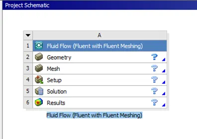
Case 1: Short Mixing Tee- applying the steps

Step 1: Pre-Processing (Geometry)

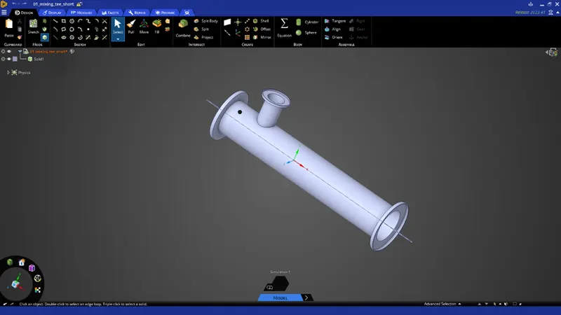
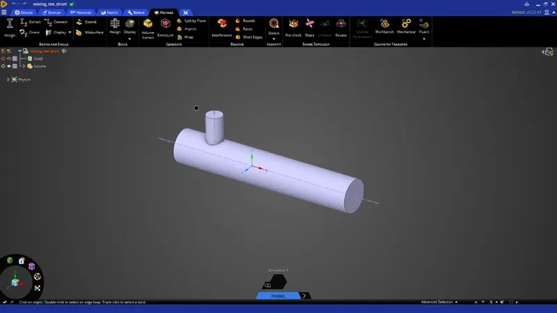
In this step, first geomery is loaded in SpaceClaim and then fluid volume extraction is done through the same. Further solid model is hide and excluded from simulation so that it will not load during further simulation process.

Step 2: Mesh

In this step follow the Watertight Geometry workflow from top to bottom as below-

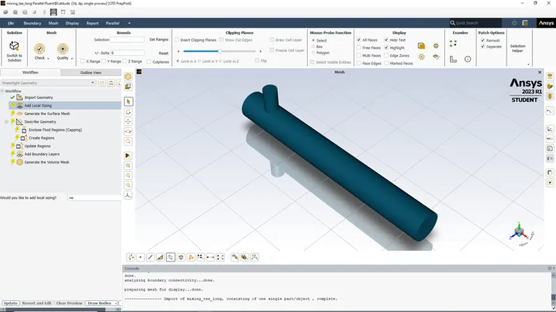
1. Import Geometry and Add Local Sizing
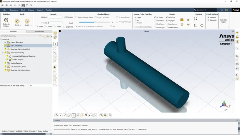
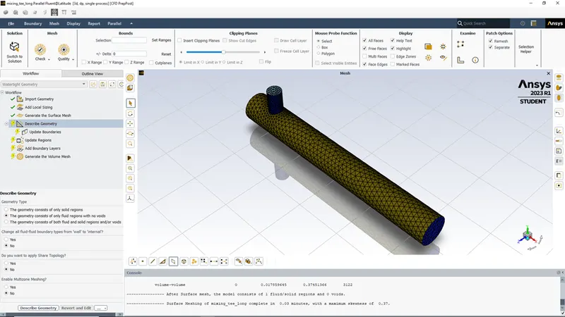
2. Generate the Surface Mesh
3. 

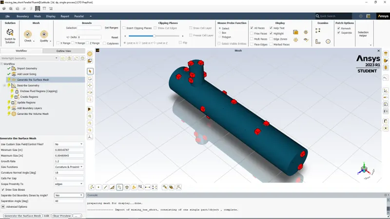
Maximum skewness is 0.32 which below 0.7 hence acceptable.

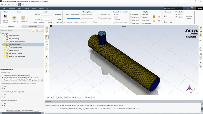
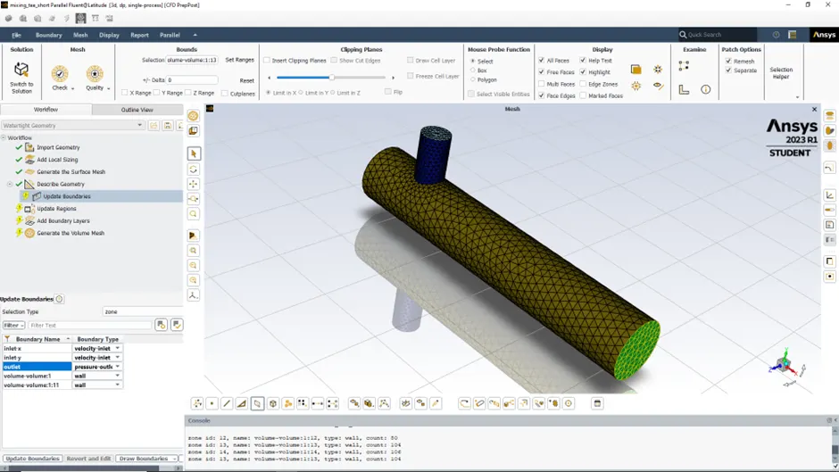
3. Describe Geometry & Update Boundaries

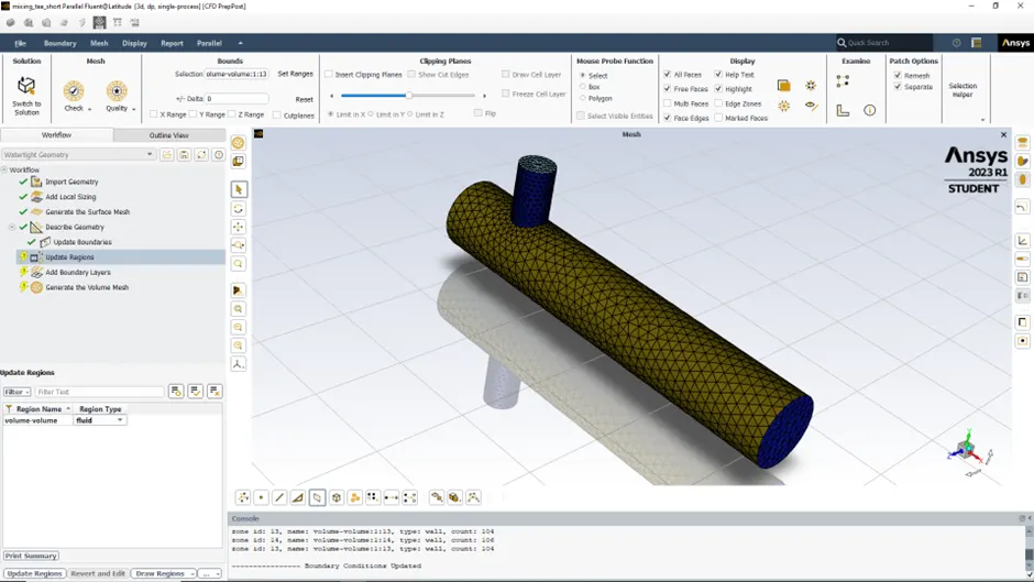
4. Update Regions

5. Add Boundary Layers

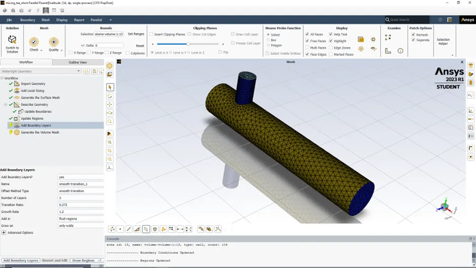
6.Generate the Volume mesh

Mesh cell size = around 0.005 m (default)

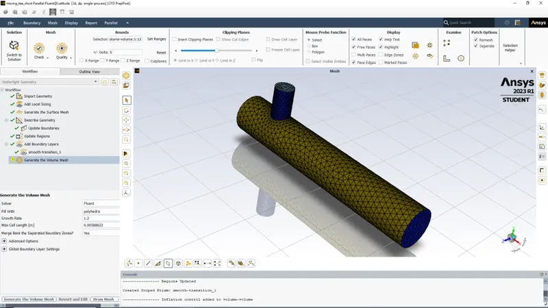
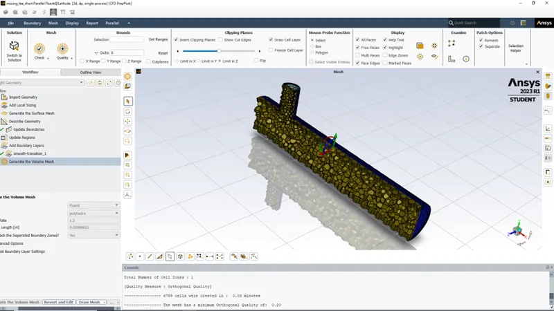
Mesh has minimum orthogonal quality of 0.20 which is more than 0.1 hence accepted.

Step 3: Setup & Solution

In this step Ribbon is used to guide the basic Fluent workflow for each cas as below-

1. Domain-

In this tab in mesh group perform mech check and evaluate mesh quality and examine the output in console.

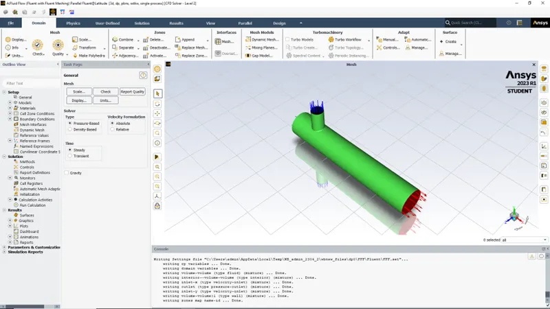
Mesh check done without error massage.

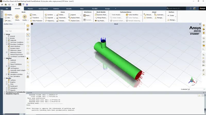
Minimum Orthogonal quality=0.20 & Aspect ratio= 10. Both orthogonal quality and aspect ratio are within acceptable range

Further in the Mesh group, click Units and select the required units

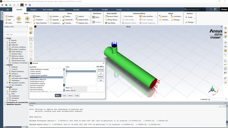2.

2. Physics- In this tab we will provide the solver, model, materials and zone sections.

First selecting the solver as Type-Pressure based and Time-steady. Also, in models select Energy to solve for temperature

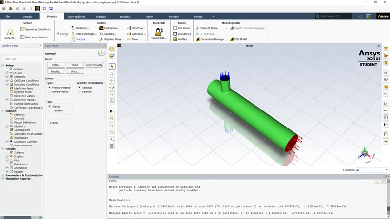
Now we will use the k-epsilon and k-omega SST model for the first case and will compare the results for following condition-

Case 1: Short Mixing Tee

1. For momentum ratio as 2 i.e.

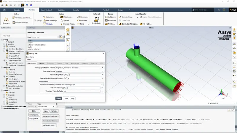
velocity at hot inlet (36⁰C)= 3m/s,

velocity at cold inlet (19⁰C)= 6m/s

a) For k-epsilon model

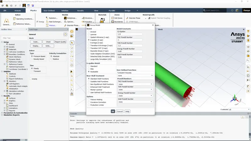
b) For k-omega SST model

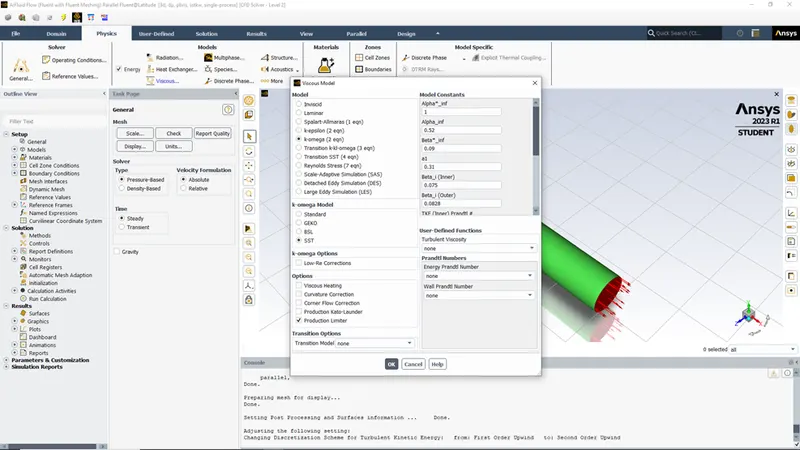
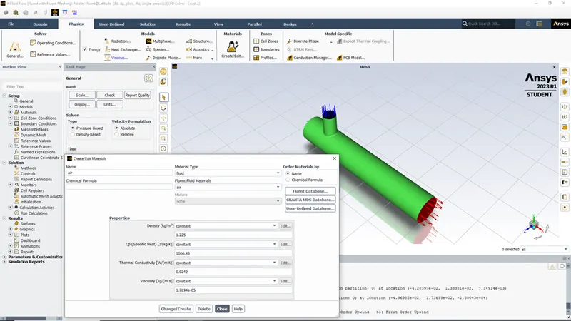
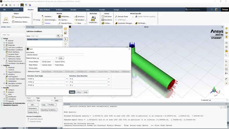
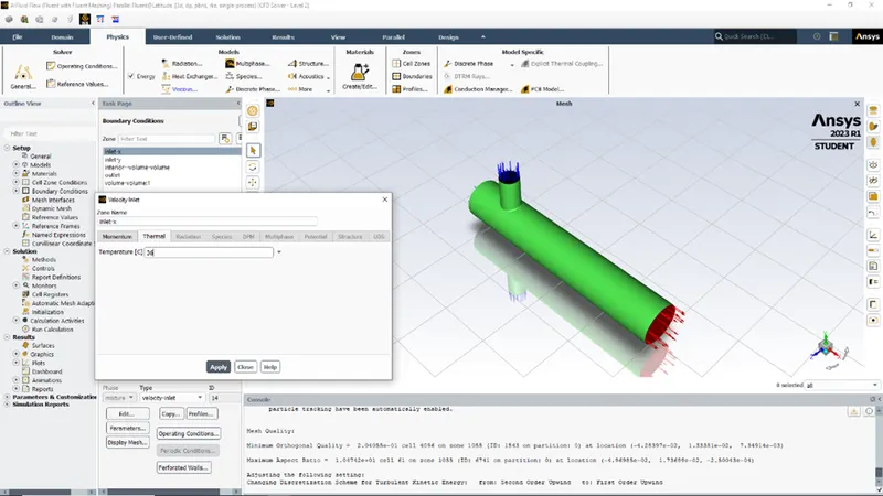
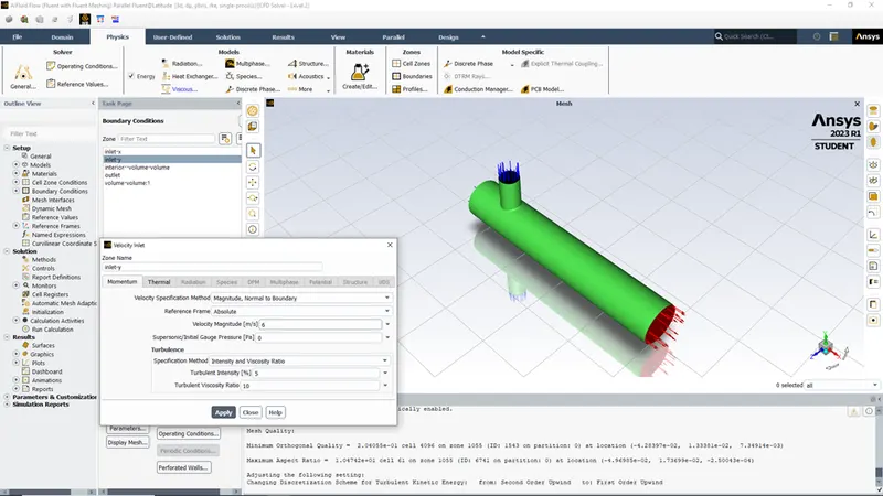
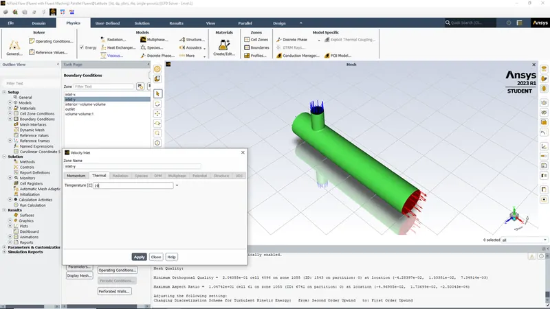
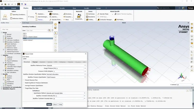
Further do the Material Selection, Zone Selection & Define Boundary Conditions for both models

Material Selection

Zone Selection

Defining Boundary Conditions

3. Solution-

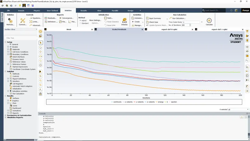
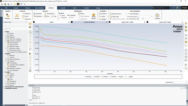
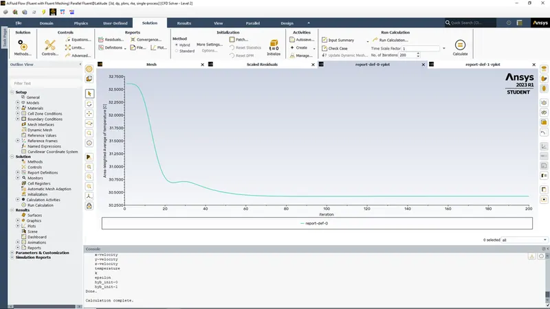
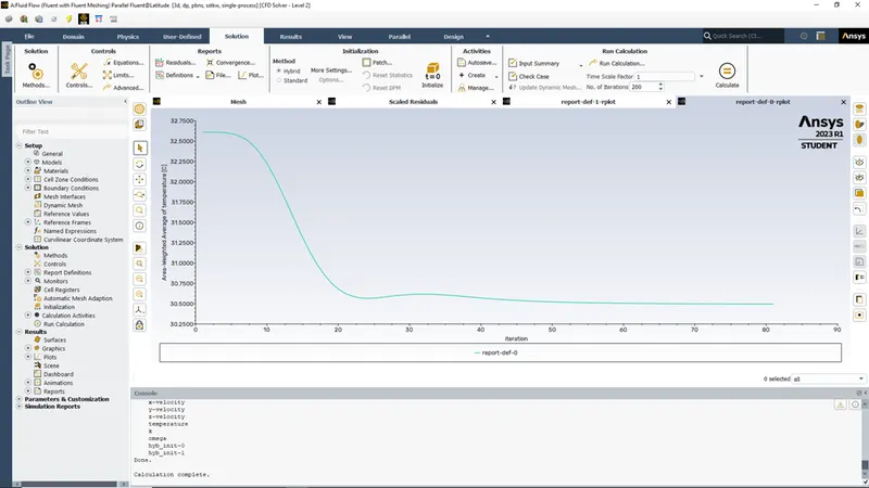
Now comparing the solution for short mixing tee with k-Epsilon and k-omega SST models for the momentum ratio of 2

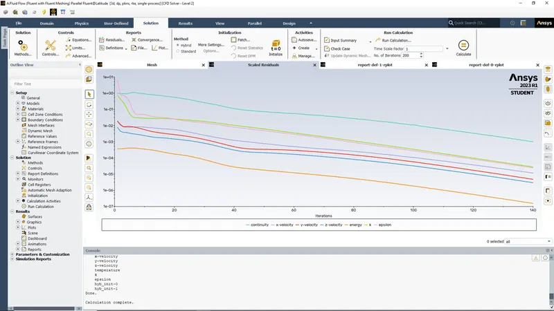
a) Residual graphs-to check the solution how much numerically accurate

For k-Epsilon model

For k-omega SST model

b) Area-weighted average temperature graphs- to get the outlet temperature

For k-Epsilon model

For k-omega SST model

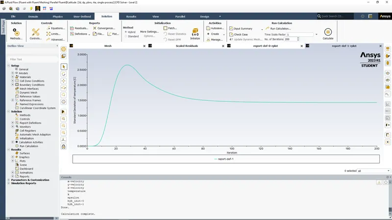
c) Standard deviation of Temperature graphs- to check the effectiveness of mixing

For k-Epsilon model

For k-omega SST model

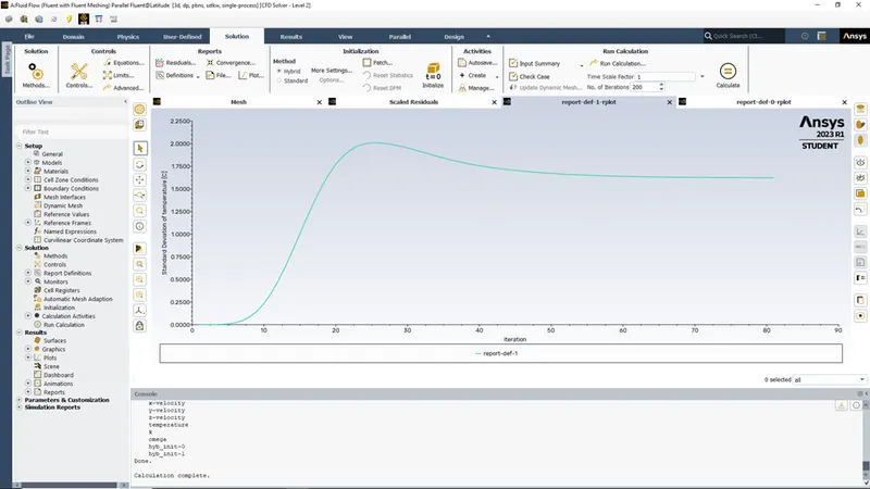
Conclusion:-

• Among the above plotted graphs, we observe much similar solutions in the Area-weighted average temperature graphs & Standard deviation of Temperature graphs for both the models. But from the residual graph we observe that for k-Epsilon model the solution converges and the plot becomes uniform after some value.
• The residual plot always shows downward slope or decreasing line means the lower the residual value is the more numerically accurate the solution.
• The standard deviation of k-Epsilon model is less than k-omega model which shows that the mixing efficiency in k-Epsilon model is better.
• K -Epsilon model predicts well far from the boundaries or walls and k - omega model predicts well near walls. Even though it depends on Y+. we also use SST model which is a combination of these
• K- epsilon model shows standard results because it becomes uniform after certain value, so we will use k-Epsilon model for all further cases.

Step 4: Post processing (Results)

Case 1: Short Mixing Tee

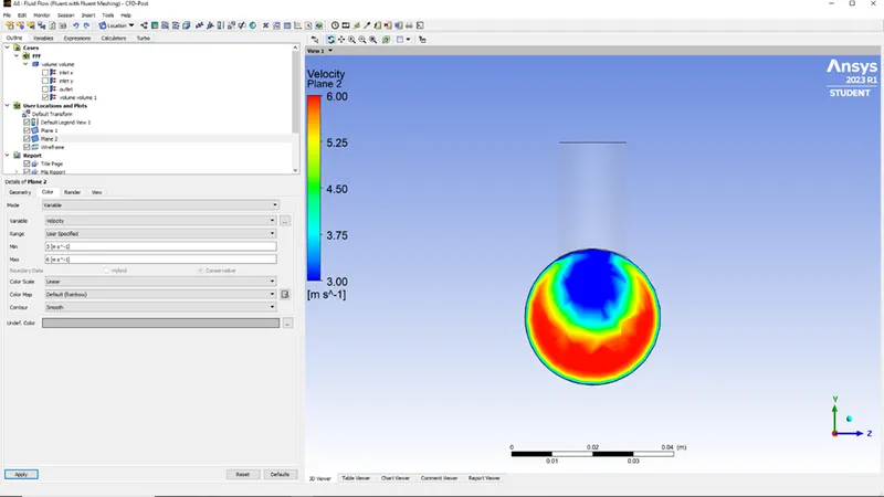
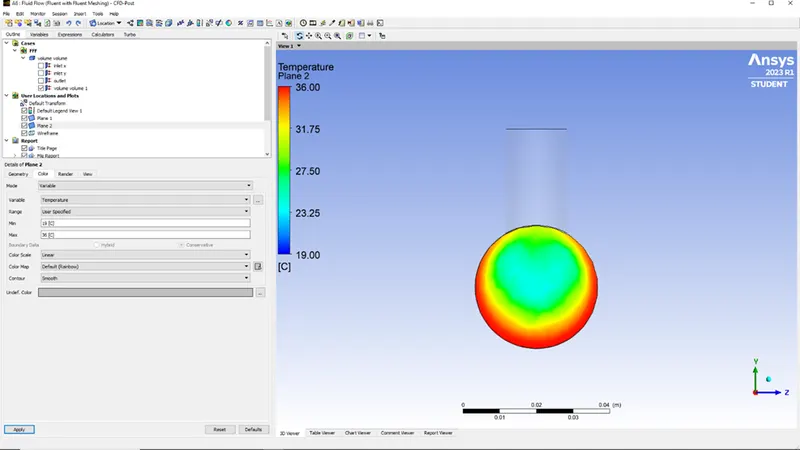
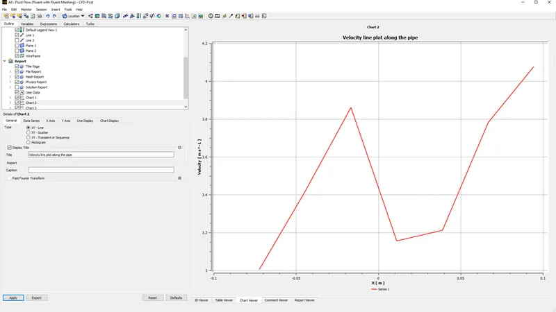
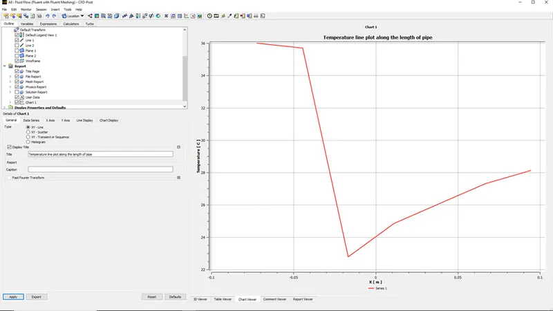
1. For momentum ratio as 2 e.

velocity at hot inlet (36⁰C)= 3m/s,

velocity at cold inlet (19⁰C)= 6m/s

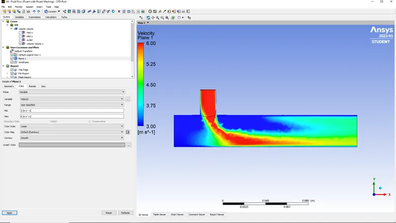
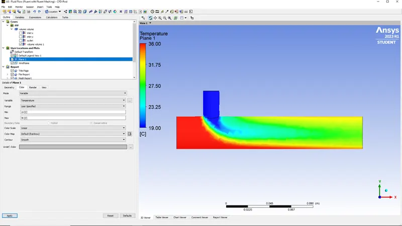
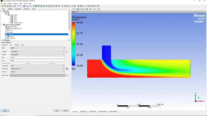
1. Velocity and temperature contour plots along the pipe

2. Velocity and temperature contour plots across the pipe

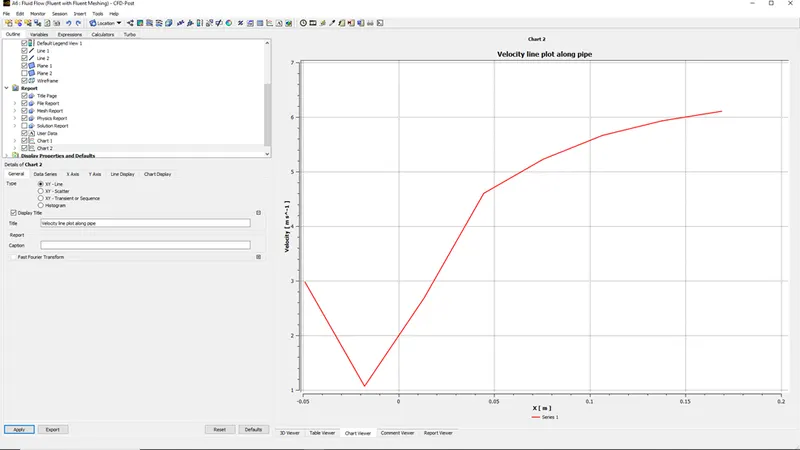
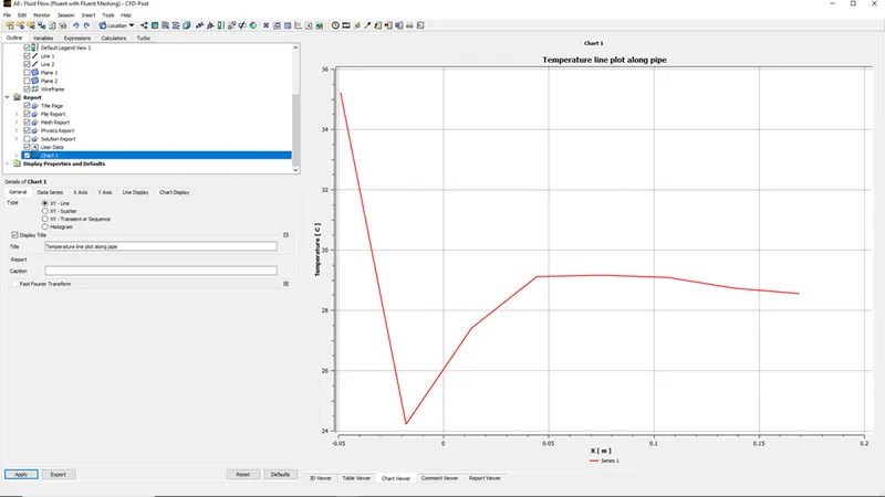
3. Velocity and temperature line plots along the pipe

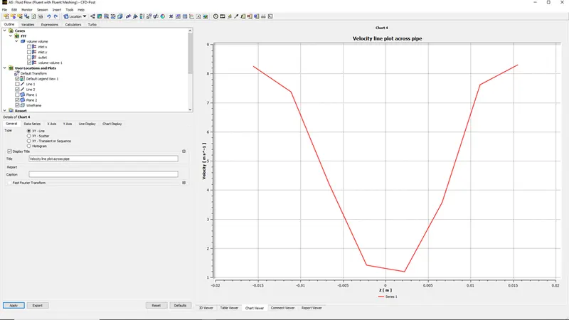
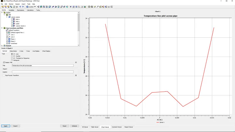
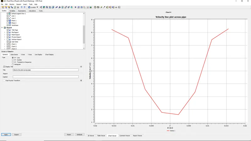
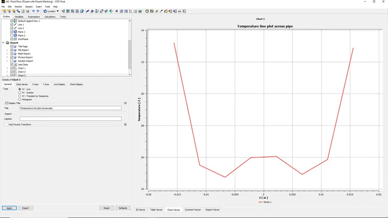
4. Velocity and temperature line plots across the pipe

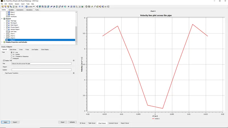
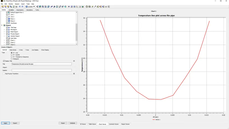
Case 1: Short Mixing Tee

2. For momentum ratio as 4 i.e.

velocity at hot inlet (36⁰C)= 3m/s,

velocity at cold inlet (19⁰C)= 12m/s

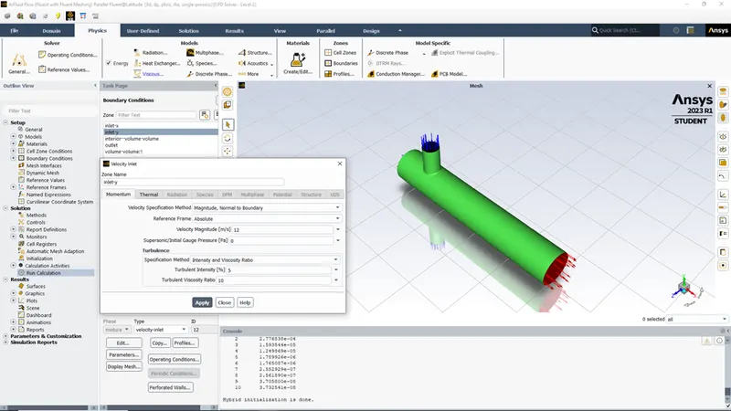
a) Residual graph-

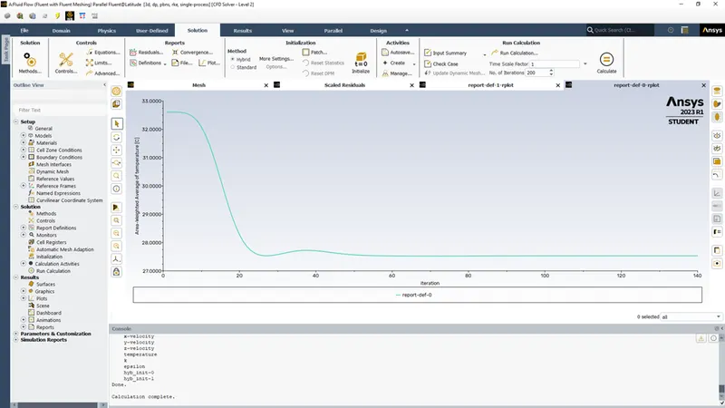
b) Area-weighted average temperature graph-

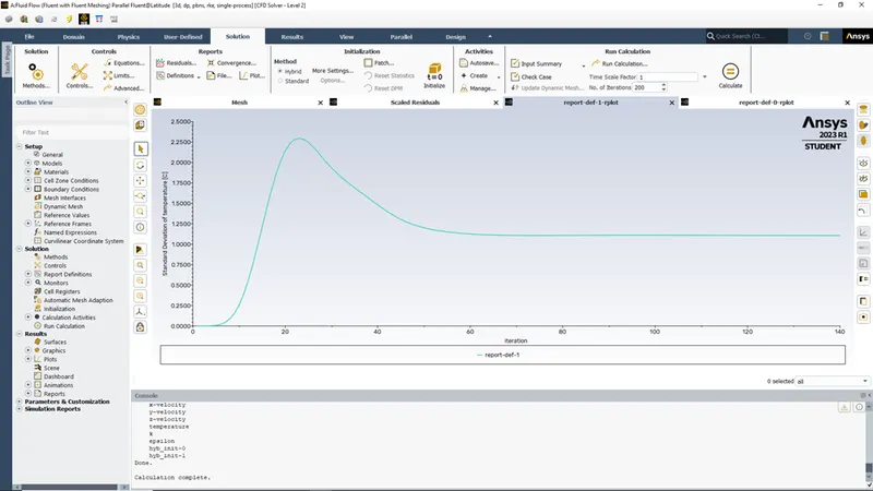
c) Standard deviation of Temperature graph-

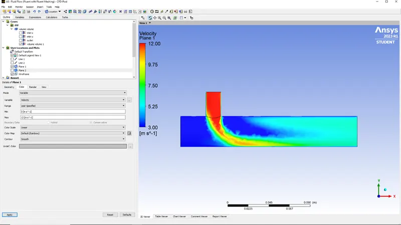
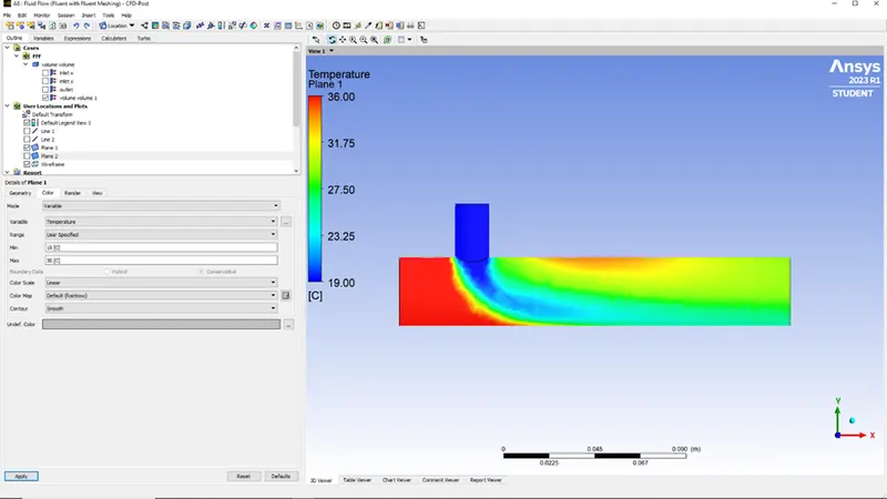
d) Velocity and temperature contour plots along the pipe

1. 

e) Velocity and temperature contour plots across the pipe

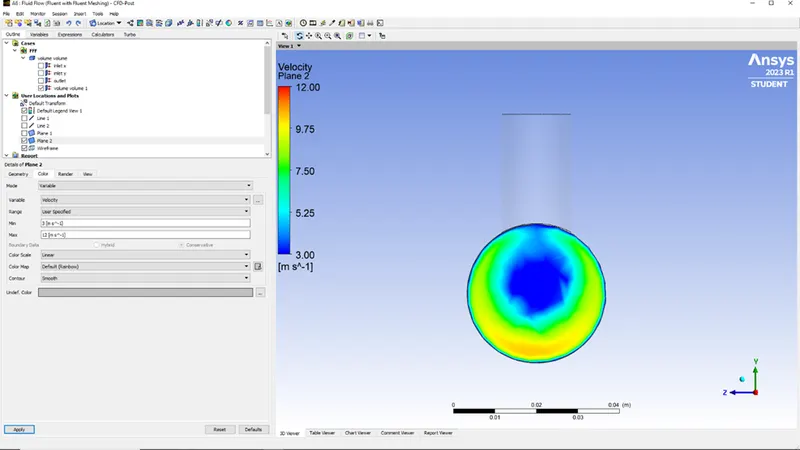
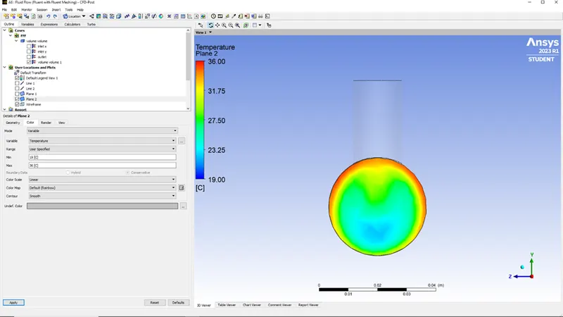
f) Velocity and temperature line plots along the pipe

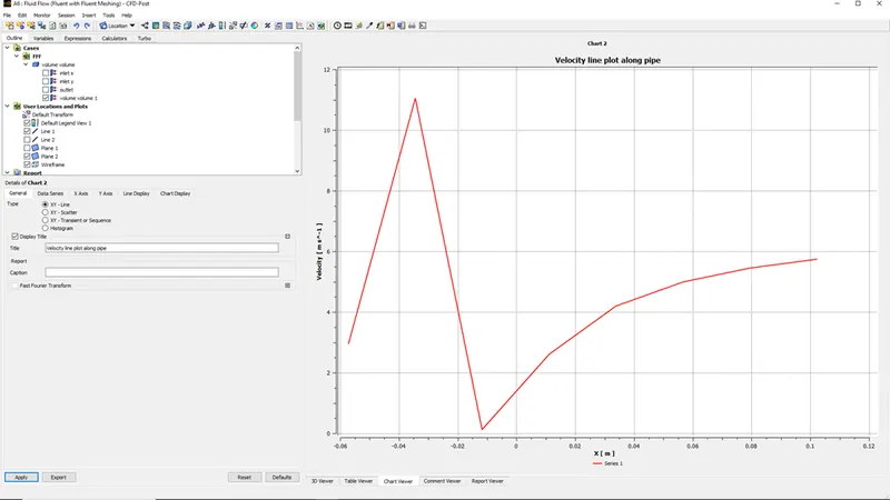
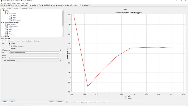
g) Velocity and temperature line plots across the pipe

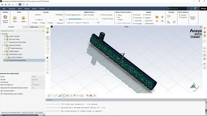
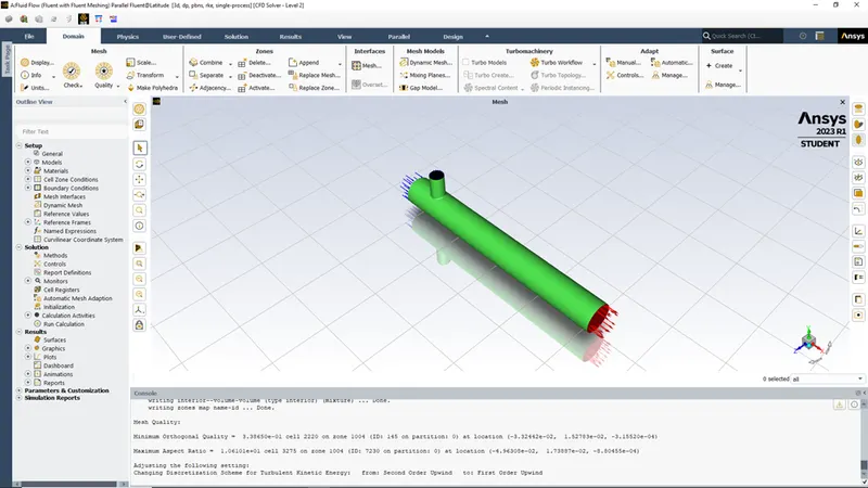
Case 2: Long Mixing Tee

1. For momentum ratio as 2 i.e.

velocity at hot inlet (36⁰C)= 3m/s,

velocity at cold inlet (19⁰C)= 6m/s

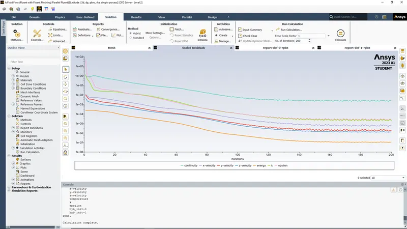
a) Residual graph-

b) Area-weighted average temperature graph-

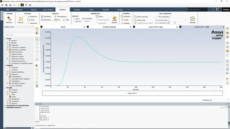
c) Standard deviation of Temperature graph-

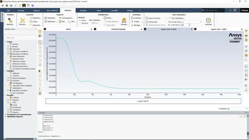
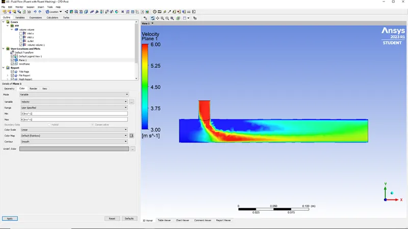
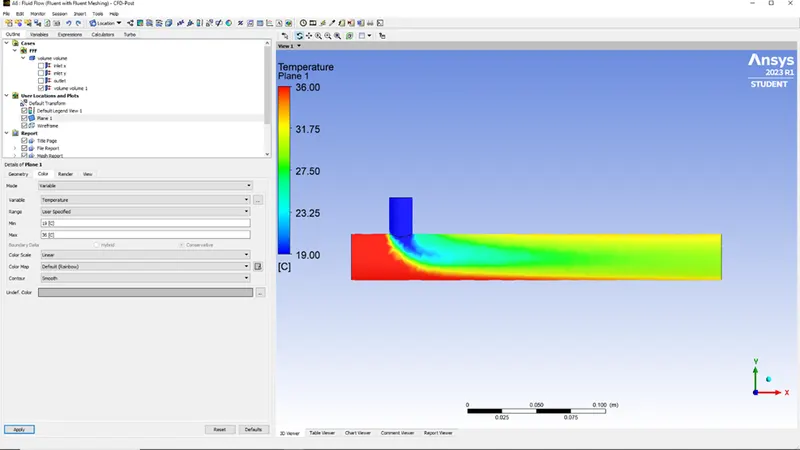
d) Velocity and temperature contour plots along the pipe

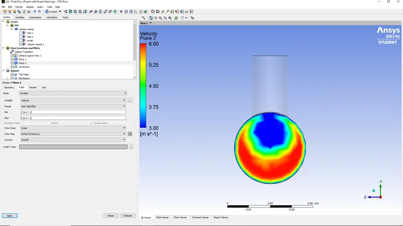
e) Velocity and temperature contour plots across the pipe

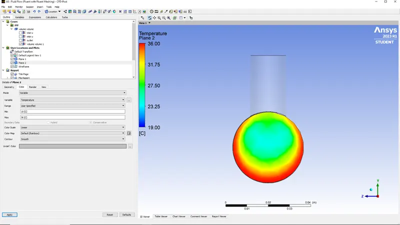
f) Velocity and temperature line plots along the pipe

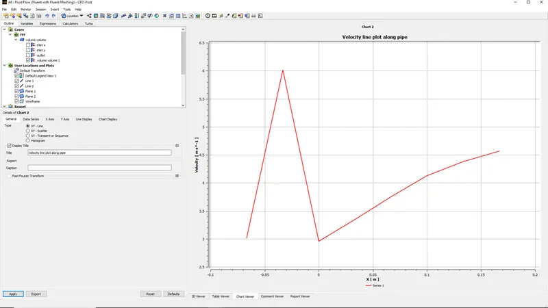
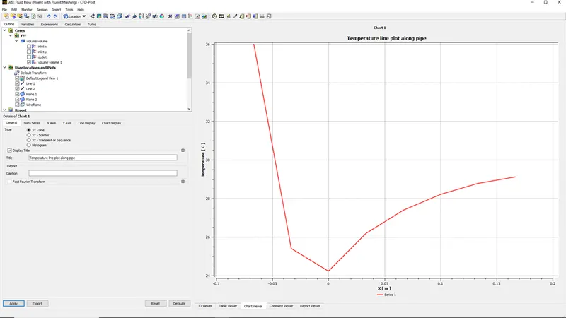
g) Velocity and temperature line plots across the pipe

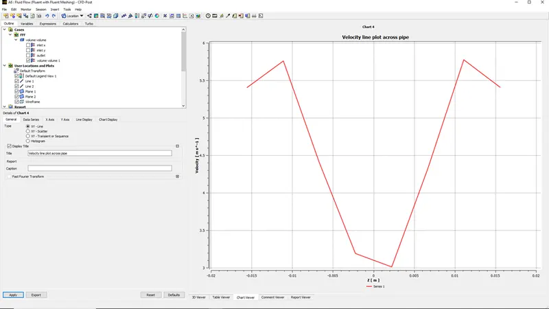
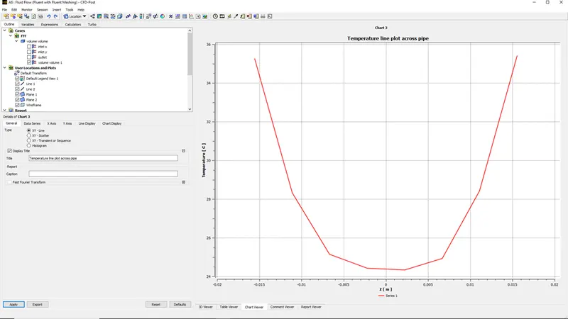
Case 2: Long Mixing Tee

1. For momentum ratio as 4 e.

velocity at hot inlet (36⁰C)= 3m/s,

velocity at cold inlet (19⁰C)= 12m/s

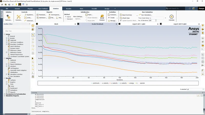
a) Residual graph-

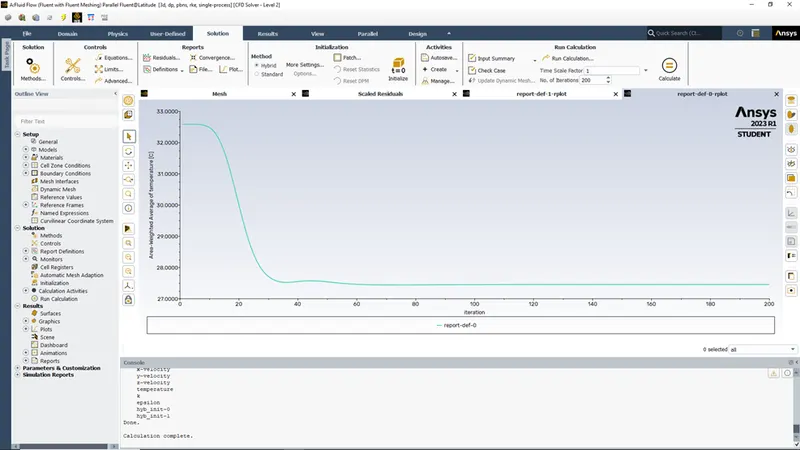
b) Area-weighted average temperature graph-

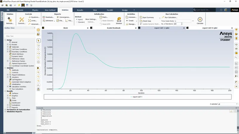
c) Standard deviation of Temperature graph-

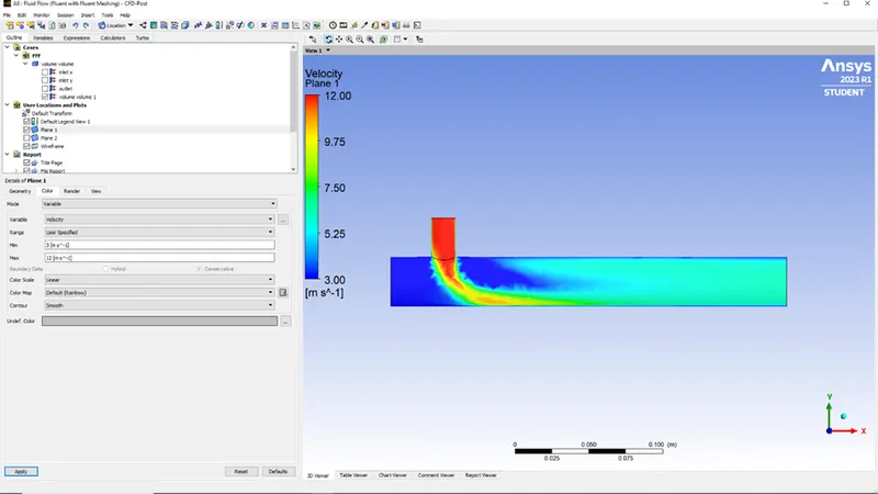
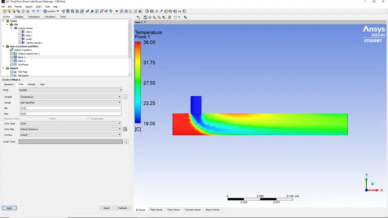
d) Velocity and temperature contour plots along the pipe

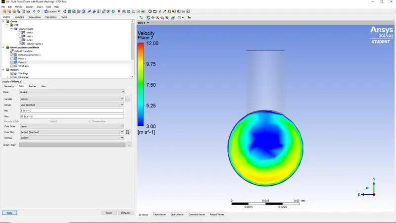
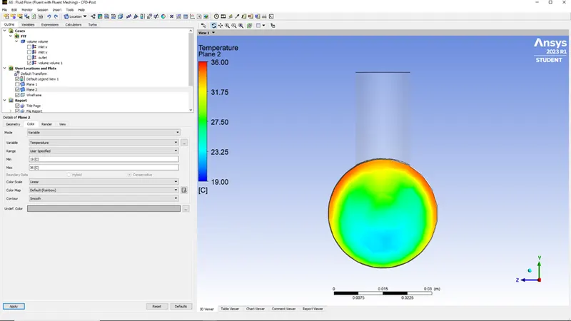
e) Velocity and temperature contour plots across the pipe

f) Velocity and temperature line plots along the pipe

g) Velocity and temperature line plots across the pipe

Summary of Results:

	Momentum Ratio	Cell Count	Avg. Outlet Temperature	No. Of iterations for convergence
Short Mixing Tee	2	6789	30.42	between 160-180
	4	6789	27.53	140
Long Mixing Tee	2	7273	30.43	between 160-180
	4	7273	27.45	between 140-160

Effect of length and momentum ratio on results

From the results it is observed that,

1. In both cases of short & long mixing tees, the average outlet temperature is nearly same for corresponding momentum ratios, it means the outlet temperature is not depended on the length of pipe
2. In both cases of short & long mixing tees, as the momentum ratio increases the average outlet temperature decreases, it means the outlet temperature is depended on momentum ratio.

Conclusion:

1. Due to increase in momentum ratio, the velocity of fluid at inlet increases and therefore when the cold & hot fluid mixes, due to high relative velocity between them causes higher turbulence and therefore the outlet temperature decreases.
2. From both contour plots it is observed that for higher momentum ratio fluids from cold & hot inlets get mixed properly due to higher turbulence i.e. for higher momentum ratio, mixing effectiveness is higher. But as compared to short mixing tee, for long mixing tee contour plots shows more uniform mixing for the higher momentum ratio.
3. Hence it is recommended to use long mixing tee with higher momentum ratio for more effective mixing.

# Mesh independence study for any one case:

Consider the case of Short Mixing Tee with momentum ratio of 2 (using k-Epsilon model)

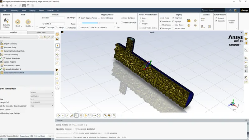
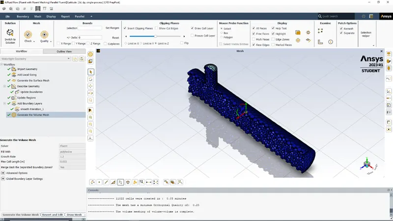
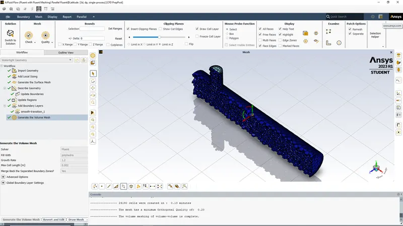
Let’s consider the following cell sizes-

1. around 0.005 m (default)
2. 003 m
3. 002 m

Cell size=around 0.005 m

Cell Size= 0.003 m

Cell Size= 0.002 m

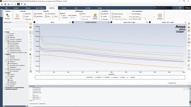
a) Residual graphs-

Cell Size =around 0.005 m

Cell Size =around 0.003 m

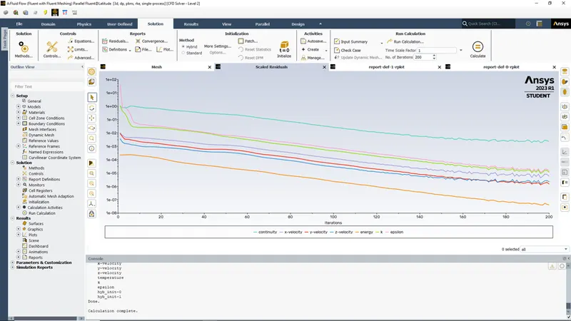
Cell Size =0.002 m

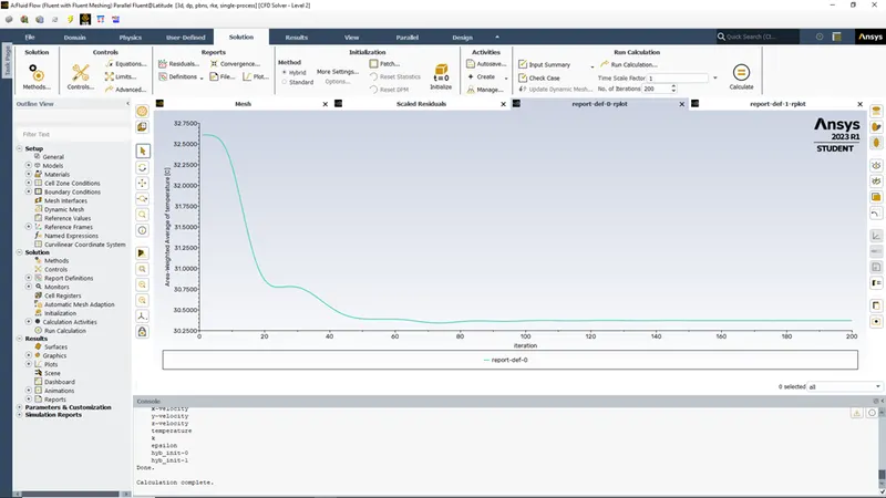
b)Area-weighted average temperature graphs-

Cell Size =around 0.005 m

Cell Size =0.003 m

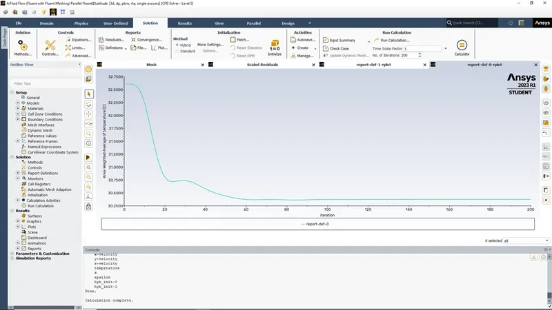
Cell Size =0.002 m

c) Standard deviation of Temperature graphs-

Cell Size =around 0.005 m

Cell Size =0.003 m

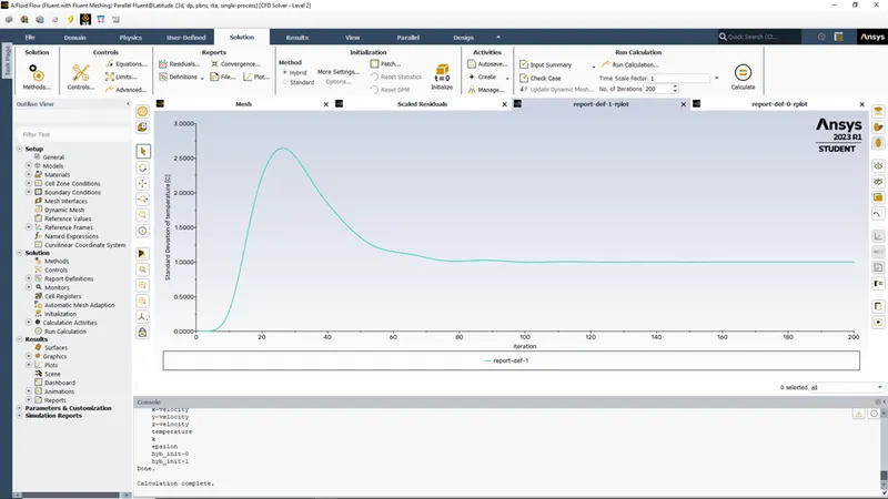
Cell Size =0.002 m

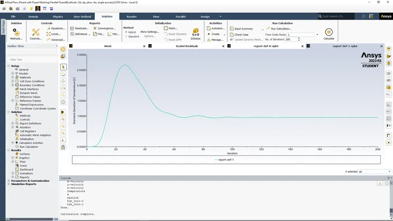
c) Velocity contour plots along the pipe-

Cell Size= around 0.005 m

Cell Size= 0.003 m

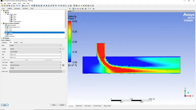
Cell Size= 0.002 m

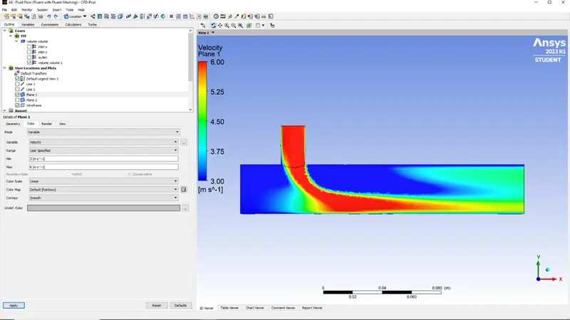
e) Temperature contour plots along the pipe-

Cell Size= around 0.005 m

Cell Size= 0.003 m

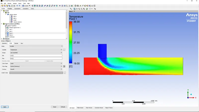
Cell Size= 0.002 m

Summary of Results:

	Cell Size	Cell Count	Min. Orthogonal Quality	Avg Outlet Temp.	Std. Deviation of Temp.
Short Mixing Tee (momentum ratio=2)	around 0.005m	6789	0.2	30.42	1.42
	0.003	11022	0.25	30.37	0.99
	0.002	24190	0.2	30.37	0.95

Conclusion-

1. As the cell size decreases, cell count increases
2. Also, with increase in cell count, simulation time get increased quadratically.
3. It is observed that as the cell count increases, solver needs more number of iterations to converge a particular value, while for lower cell count, solver converges fast.
4. The velocity & temperature Contour plots are sharper for lower cell count while as the cell count increases contour plots become finer.