Week 2 - Flow over a Cylinder.

Aim: To simulate the flow over a cylinder and explain the phenomenon of Karman vortex street.   

Objective:

1. The major objective of this project is to perform a two-dimensional flow analysis over a cylinder for a particular Reynolds number, to observe and study the phenomenon of vortex shedding. The analysis is carried out for both steady and transient state conditions.
2. Also for steady state condition, calculate the coefficient of drag and lift over the cylinder for different Reynolds number and check the effect of Reynolds number on coefficient of drag

Theory:

Vortex Shedding-

Vortex shedding is an oscillating flow that takes place when a fluid such as air or water flows past a bluff (as opposed to streamlined) body at certain velocities, depending on the size and shape of the body. In this flow, vortices are created at the back of the body and detach periodically from either side of the body forming a Kármán vortex street. The fluid flow past the object creates alternating low-pressure vortices on the downstream side of the object. The object will tend to move toward the low-pressure zone.Under the correct flow conditions, the flow around a bluff body produces a regular pattern of alternating vortices known as a von Karman vortex street . These vortices produce a sinusoidal force acting on the body perpendicular to the flow.

                                     

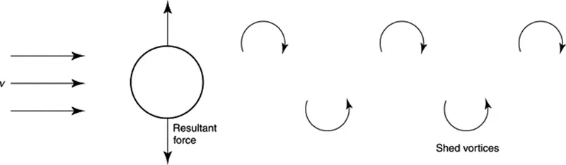
                                                                               Figure. Vortex shedding.

For a cylinder, the frequency f (in Hz) of the shedding is related to the diameter D(m) and wind speed v (ms⁻¹) via dimensionless number called Strouhal number St, such that

                                                                                       

If the frequency of the shed vortices is the same as one of the natural frequencies of the structure, then large vibrations can result. Although it is possible for this loading to cause the structure to fail through the ultimate load being exceeded, failure is more likely to occur through fatigue. The effect is exacerbated by an effect known as ‘lock-in’ where the vortex shedding frequency is forced to remain at the critical structural frequency at a range of speeds below and above the critical speed.

 Importance in Practical Application-

 The design of bridges, chimneys, submarine periscopes, etc. must take this phenomenon into account. Aerodynamic devices are used commonly nowadays to either ensure that the flow remains attached, or to break up the regular formation of the vortexes.

References:-

https://en.wikipedia.org/wiki/Vortex_shedding

https://doi.org/10.1006/rwvb.2001.0125

Solution: To set up the simulation in each case steps followed are as below-

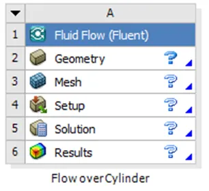
Step 1: Pre-Processing (Geometry)

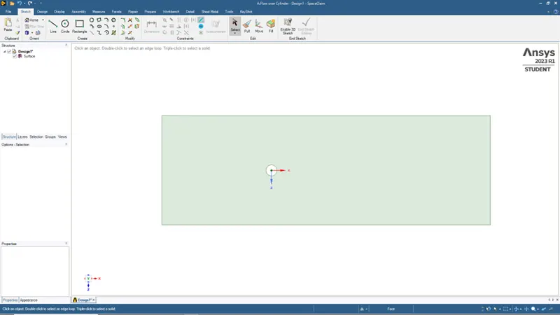
In this step, we will create 2D geometry in SpaceClaim

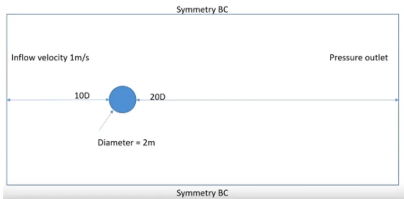
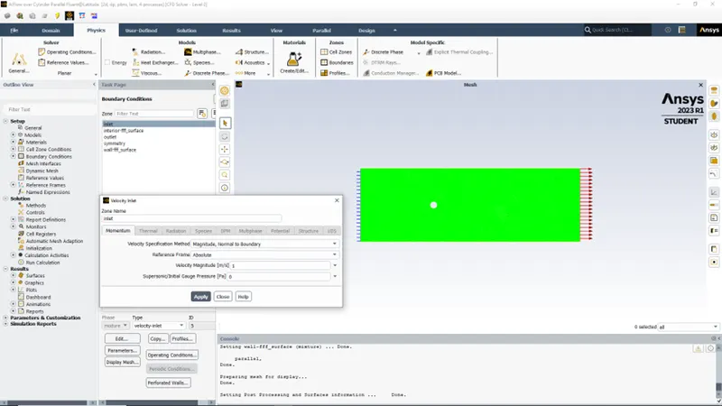
In the above sketch, there is a 2D cylinder which is immersed in the fluid domain having the inlet flow velocity of 1 m/s and pressure outlet is 1 atm.

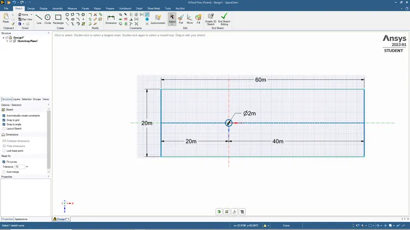
Then convert the geometry into surface

Step 2: Mesh

Ansys creates quadrilateral mesh of default size.

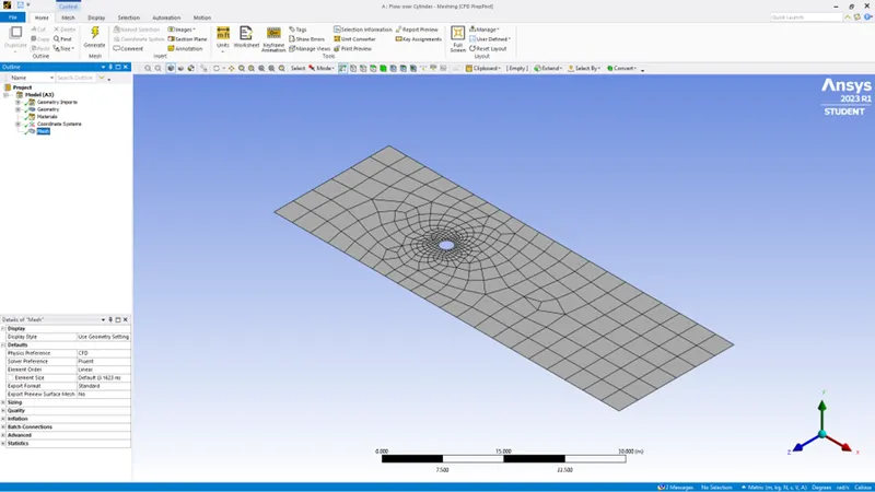
We will change the default mesh to triangular mesh

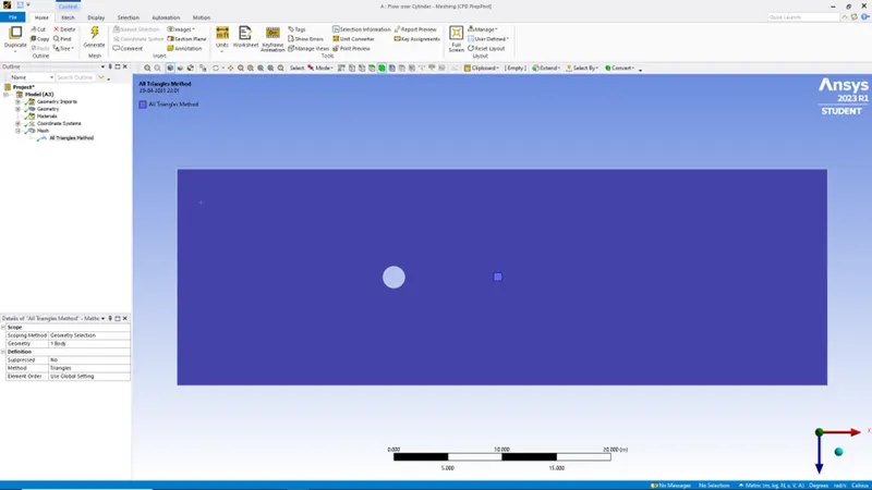
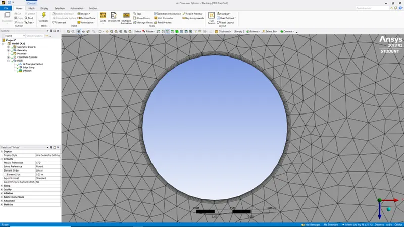
We generate the triangular mesh with element size of 0.25 m

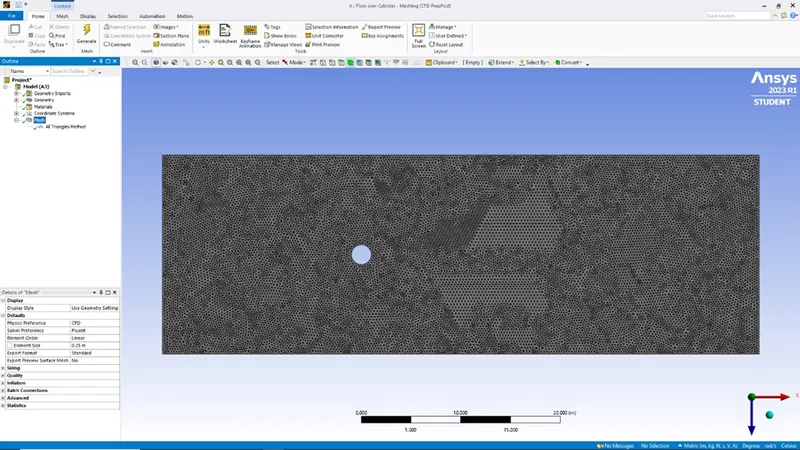
To make the perfect cylindrical boundary, the sharp corners around the circle are divided into large number of edges by Edge Sizing.

Number of divisions selected as 36

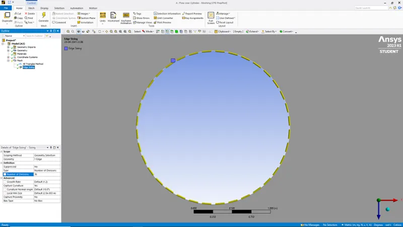
Since the flow over cylinder is important, the inflation layer is created around the cylinder boundary

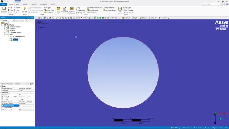
To create the inflation layer, First Layer Thickness method is used with –

First layer thickness = 0.005 m

Maximum layers = 6

Growth rate = 1.2

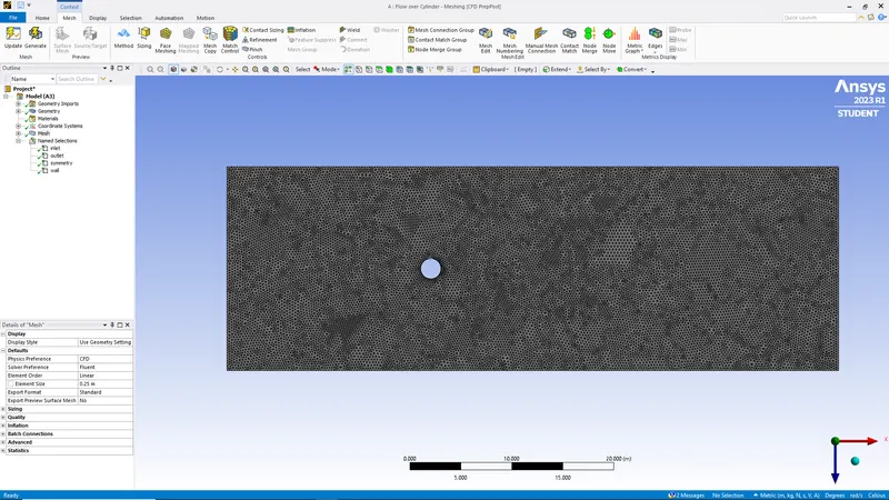
Final mesh is created by providing named selections to the boundary conditions as inlet, outlet, wall & symmetry

Step 3: Setup & Solution

Part 1:  Simulate the flow with steady & transient case and calculate the Strouhal number for Re=100

Case 1: Steady State & Re=100

1. Physics- In this tab we will provide the solver, model, materials and zone sections.

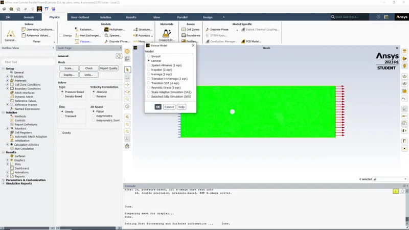
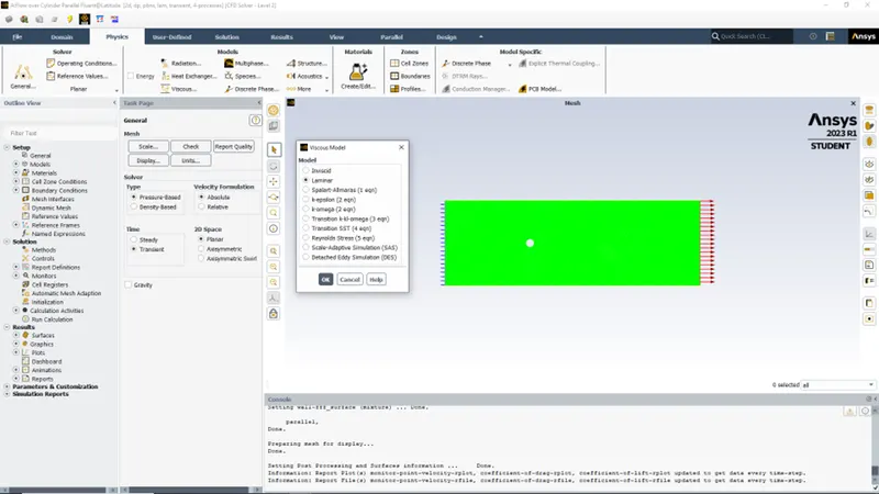
 First selecting the solver as Type-Pressure based and Time-steady.

Also, in viscous models select Laminar to solve the flow for lower Re i.e. Re < 2000

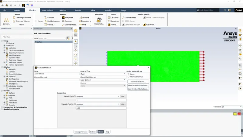
Material Selection– For given condition of Re=100, V= 1m/s & D= 2 m,

Selecting the material as User-Defined with Density=1 kg/m³ & viscosity =0.02 kg/ms

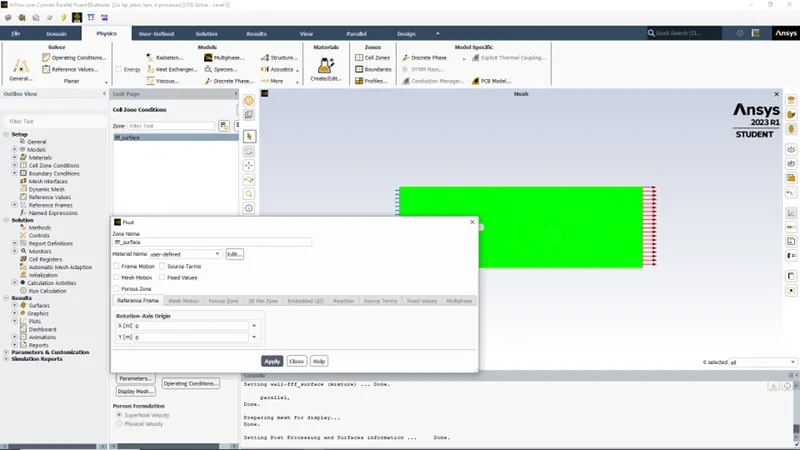
Zone Selection

Defining Boundary Conditions

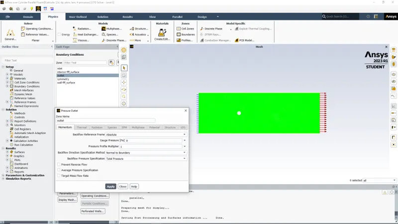
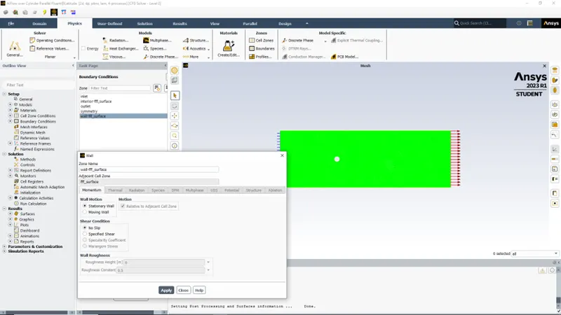
2. Solution

 After that we will create monitor-point (behind the cylinder at a distance 4D i.e. 8m from the centre of cylinder along x-direction) where we want to capture flow pattern or Vortex shedding

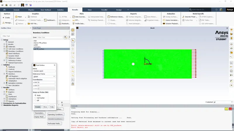
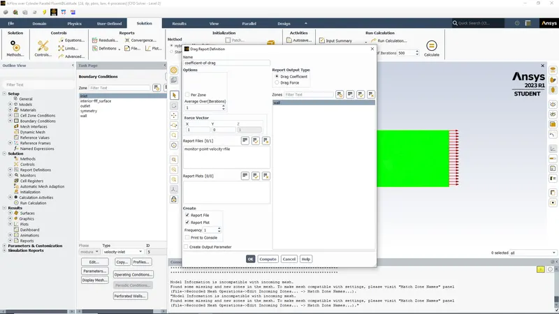
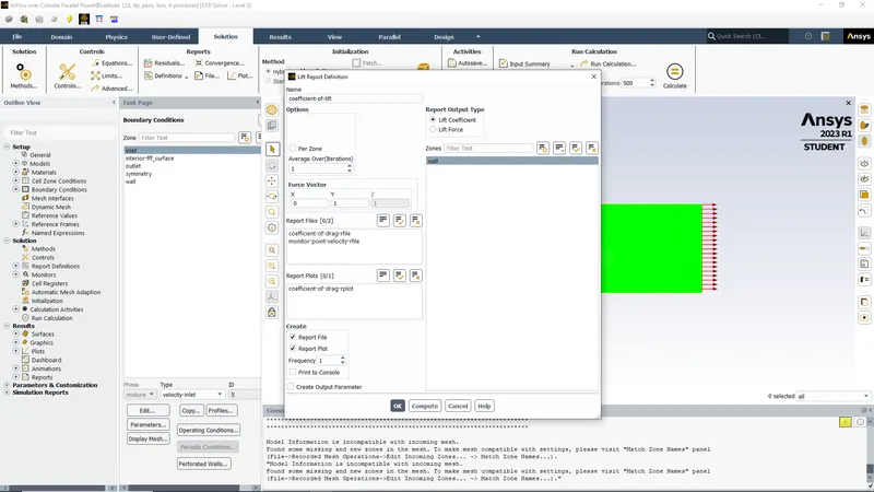
Then surface reports are created to measure velocity average of monitor point, coefficient of drag & coefficient of Lift

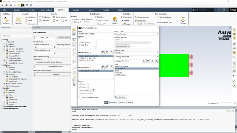
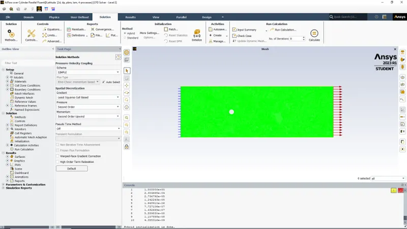
Solution Method- selected as SIMPLE

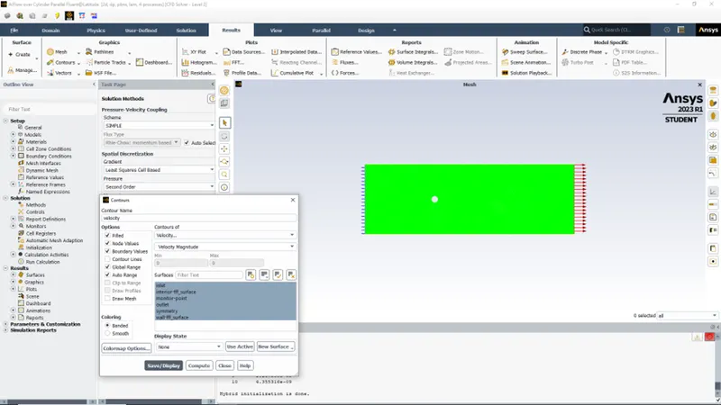
Also contour plots are created for velocity & pressure

Results for Steady State Simulation-For Re=100

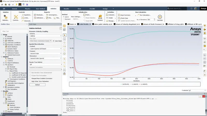
• Residual Plot

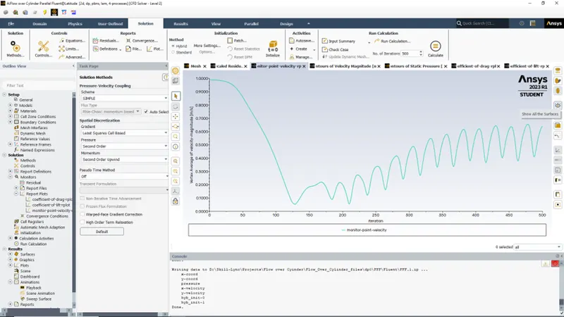
• Vertex Average of Velocity Magnitude

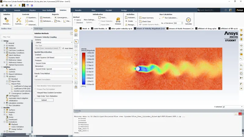
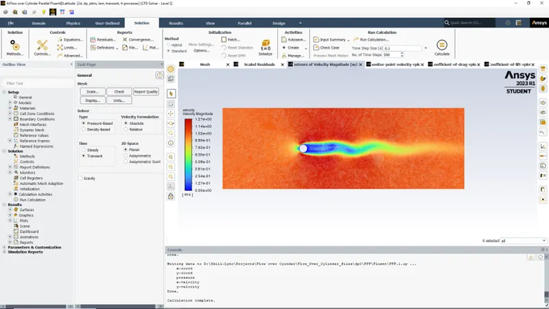
• Velocity Contour Plot

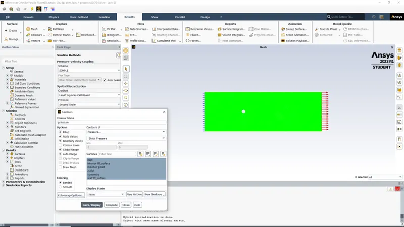
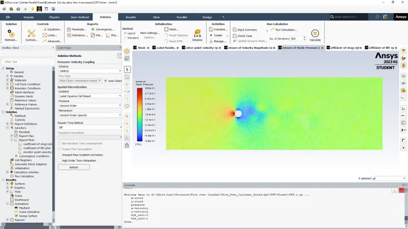
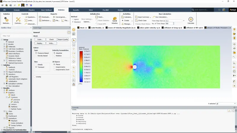
• Pressure Contour Plot

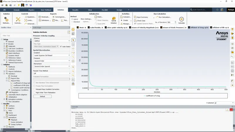
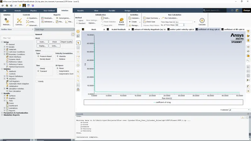
• Coefficient of Drag

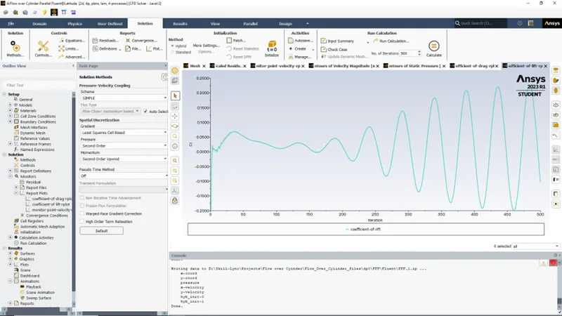
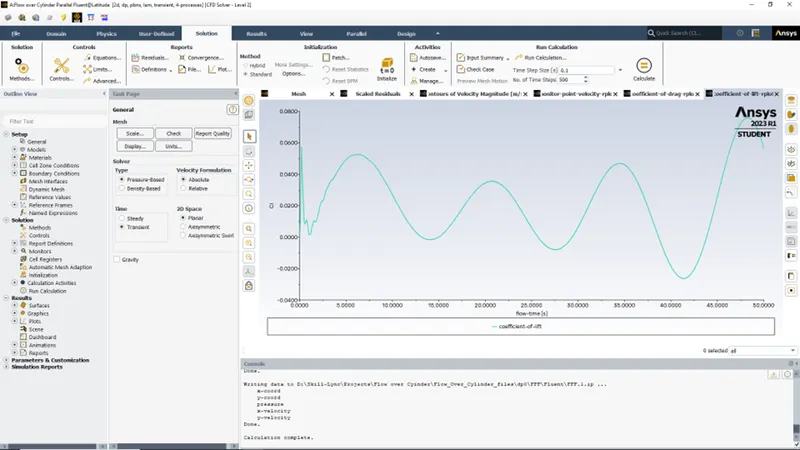
• Coefficient of Lift

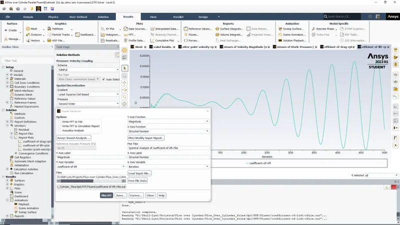
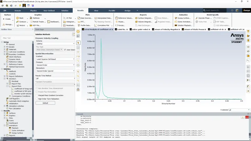
• Strouhal Number Plot

Strouhal Number is obtained from FFT plot, in which take magnitude on y-axis and Strouhal Number on x-axis and then load file of coefficient of lift.

Case 2: Unsteady State & Re=100

Results for Steady State Simulation-For Re=100

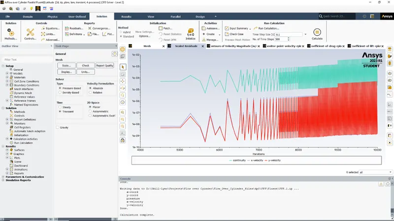
• Residual Plot

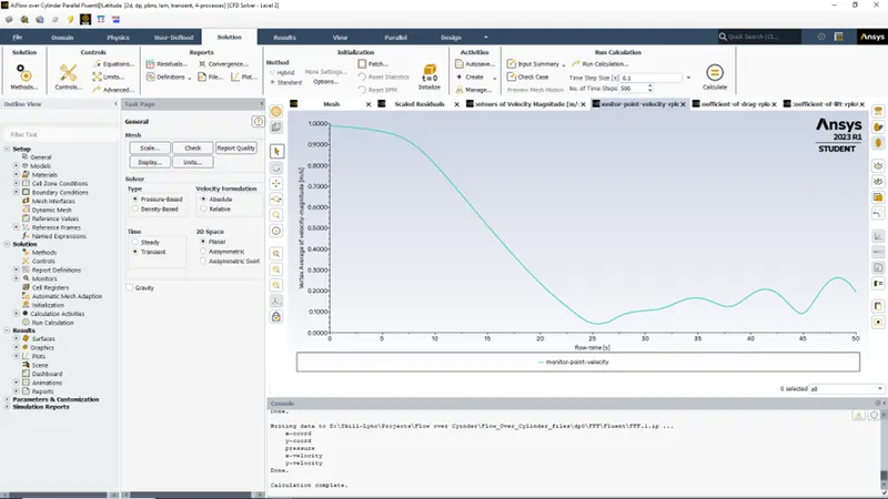
• Vertex Average of Velocity Magnitude

• Velocity Contour Plot

• Pressure Contour Plot

• Coefficient of Drag

• Coefficient of Lift

• Strouhal Number Plot

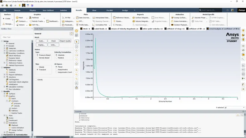
Summary of Results:

	Reynolds No. (Re)	Strouhal Number (Sr)
Steady State	100	0.0205
Unsteady State	100	0.0755

Conclusion:

A) For Steady state condition

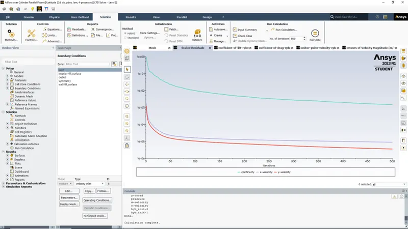
1. From the residual plots it is observed that, the error values are not changing with iterations & become steady after 350 iterations, hence we can conclude that the solution is converged.
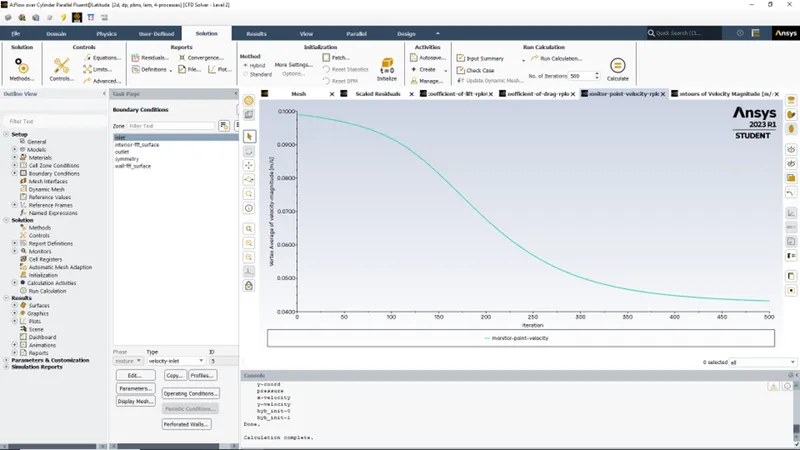
2. From the velocity plot it is observed that, the oscillations start after 200 iterations which means formation of vortices takes place.
3. From the velocity contour plot it is seen that, the velocity is almost zero for the first few layers around the cylinder due to no-slip boundary condition. But the velocity is almost equal to free stream velocity of 1 m/s in the adjacent layers. So, the high velocity gradient causes separation of flow from the body which tends to rotate the fluid elements. Since this phenomenon takes place on both sides of cylinder, the alternate rotations cause formation of vortices (also seen in the plot).
4. From the pressure contour plot it is seen that the pressure is maximum at front side (left) of the cylinder due to the impact of fluid on the cylinder. Also the alternatively changing low pressure field is observed behind (right) of the cylinder which means that the low pressure wake region is formed.

 B) For Unsteady state condition

1. From the residual plots it is observed that, the amplitude of oscillations of residuals become steady after 9000 iterations, hence we can say the solution is converged.
2. From the velocity plot it is observed that, the oscillations start after after 25 sec which means formation of vortices takes place.
3. From the velocity & pressure plots phenomenon of vortex shedding & formation of low pressure wake region can be observed.

              Since in real world, vortex shedding phenomenon depends on time, it is better to use transient solver to simulate this problem. But in transient mode, more iterations are required to develop proper physics of the flow. Because of that the transient simuation has taken more iteration with smaller time steps compare to the steady state. 

Part 2: Calculate the coefficient of drag and lift over a cylinder by setting the Reynolds number to 10,100,1000,10000 & 100000

Case 1: Re=10

For given condition of Re=10, D= 2 m,

Keeping the material as User-Defined with Density=1 kg/m³ & viscosity =0.02 kg/ms

Changing boundary condition for inlet as Velocity= 0.1 m/s

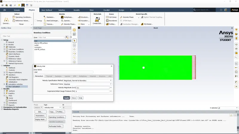
Results for steady state simulation for Re=10

• Residual Plot

• Vertex Average of Velocity Magnitude

• Velocity Contour Plot

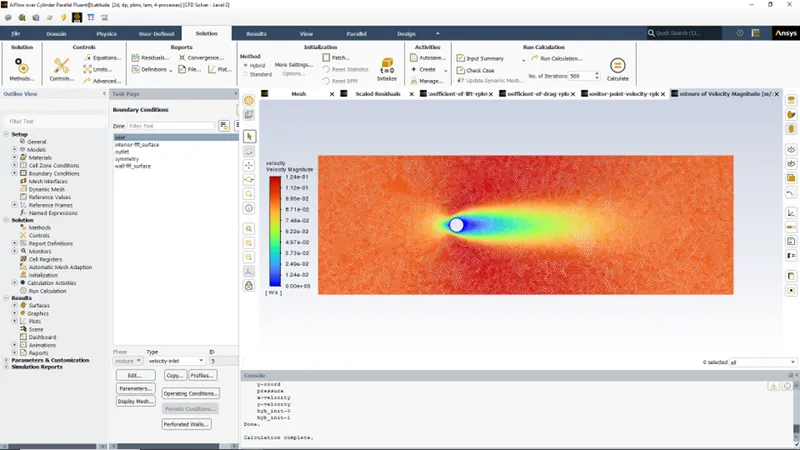
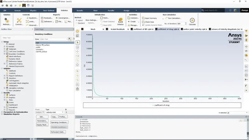
• Coefficient of Drag

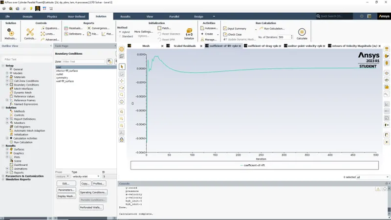
• Coefficient of Lift

Case 2: Re=100

For given condition of Re=10, D= 2 m,

Keeping the material as User-Defined with Density=1 kg/m³ & viscosity =0.02 kg/ms

Changing boundary condition for inlet as Velocity= 1 m/s

Results for Steady State Simulation-For Re=100

• Residual Plot

• Vertex Average of Velocity Magnitude

• Velocity Contour Plot

• Coefficient of Drag

• Coefficient of Lift

Case 3: Re=1000

For given condition of Re=10, D= 2 m,

Keeping the material as User-Defined with Density=1 kg/m³ & viscosity =0.02 kg/ms

Changing boundary condition for inlet as Velocity= 10 m/s

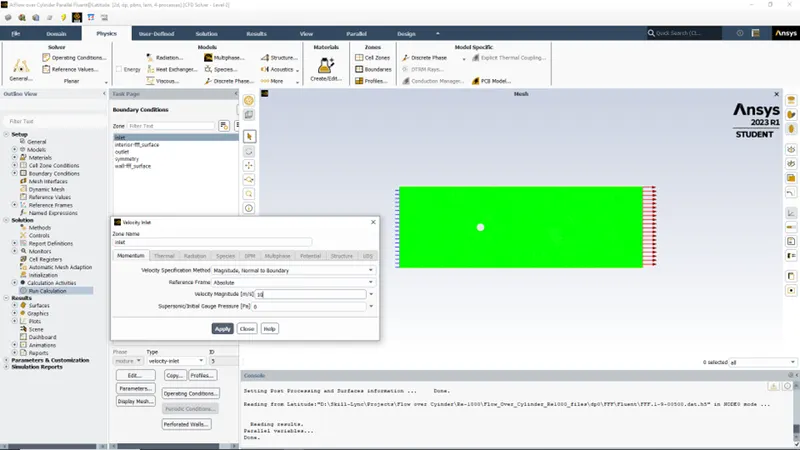
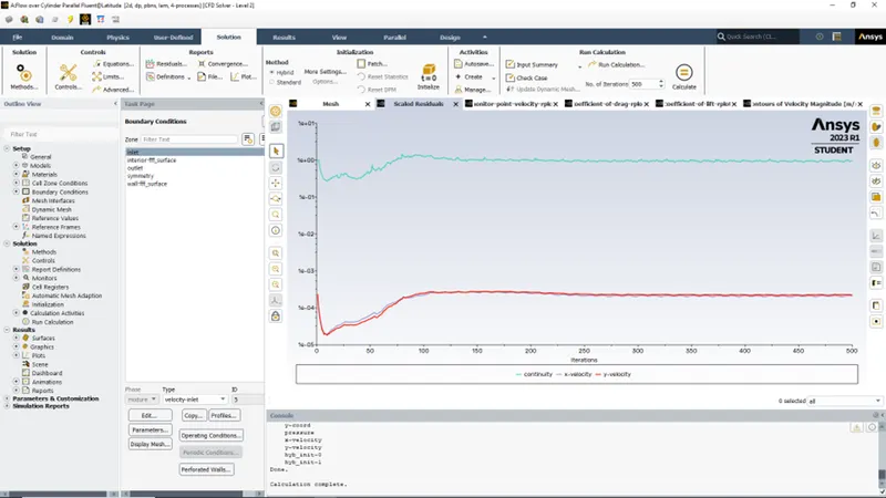
Results for Steady State Simulation-For Re=1000

• Residual Plot

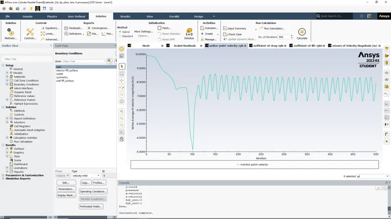
• Vertex Average of Velocity Magnitude

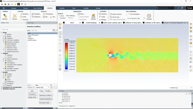
• Velocity Contour Plot

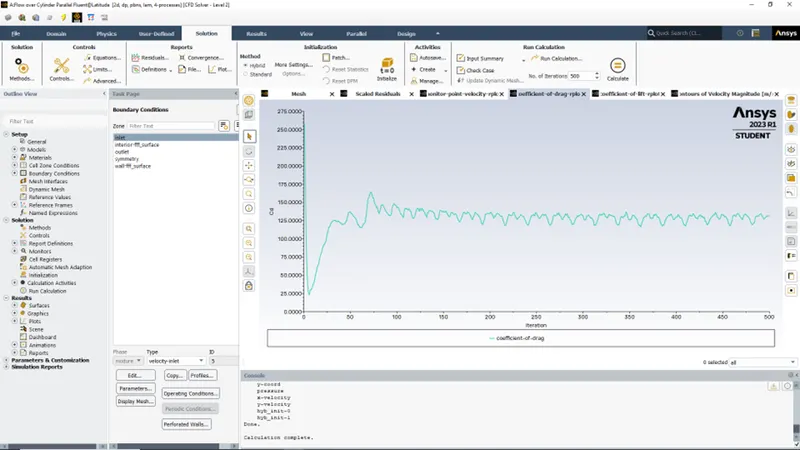
• Coefficient of Drag

• Coefficient of Lift

Case 4: Re=10000

For given condition of Re=10, D= 2 m,

Keeping the material as User-Defined with Density=1 kg/m³ & viscosity =0.02 kg/ms

Changing boundary condition for inlet as Velocity= 100 m/s

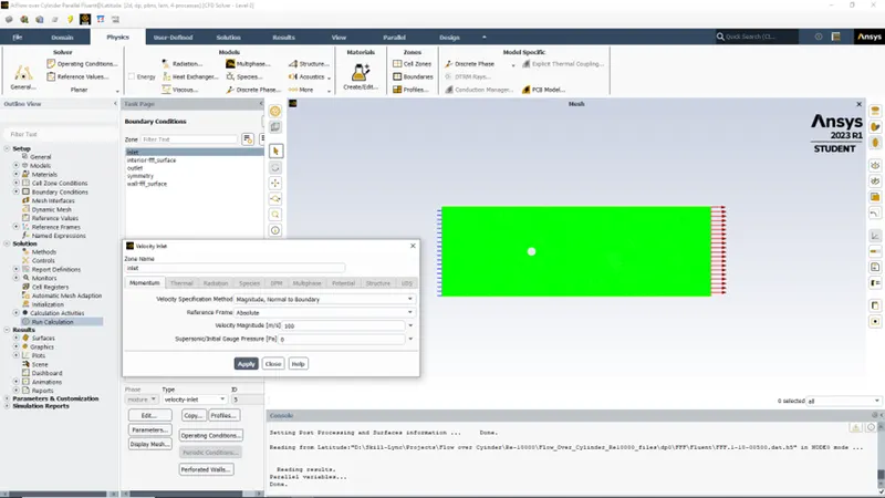
Results for Steady State Simulation-For Re=10000

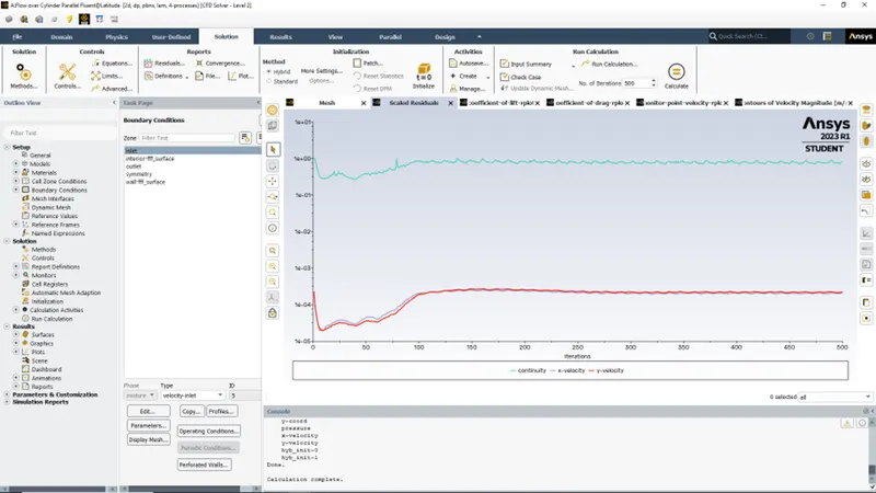
• Residual Plot

• Vertex Average of Velocity Magnitude

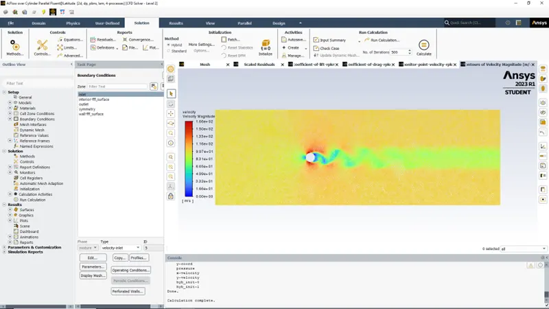
• Velocity Contour Plot

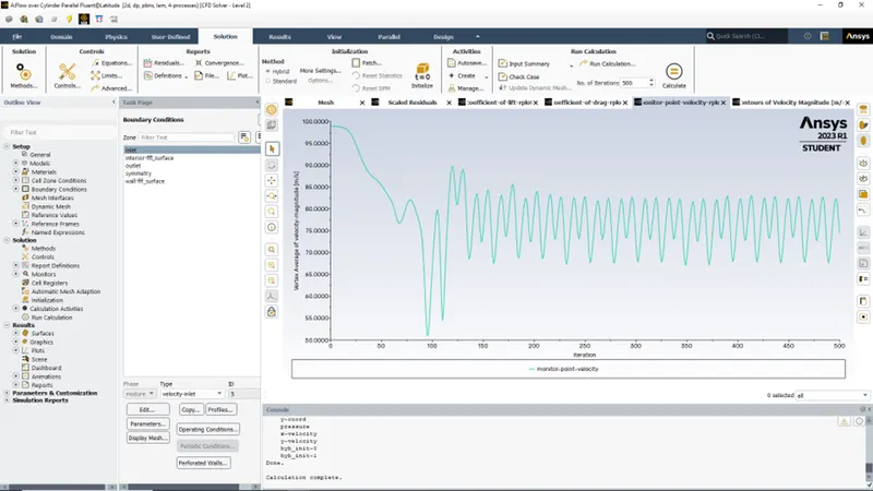
• Coefficient of Drag

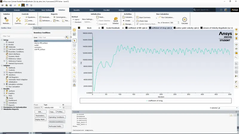
• Coefficient of Lift

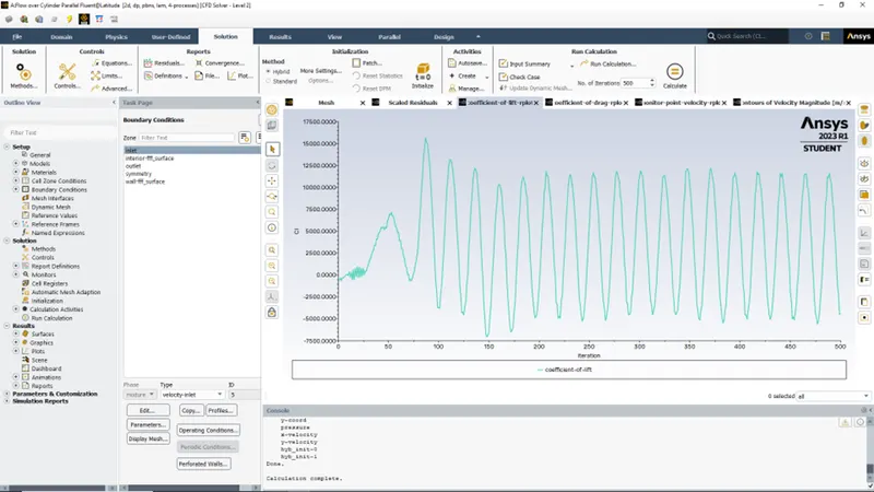
Case 4: Re=100000

For given condition of Re=10, D= 2 m,

Keeping the material as User-Defined with Density=1 kg/m³ & viscosity =0.02 kg/ms

Changing boundary condition for inlet as Velocity= 1000 m/s

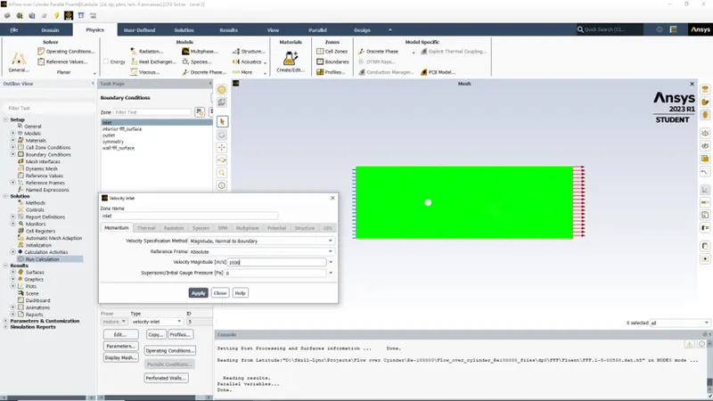
Results for Steady State Simulation-For Re=100000

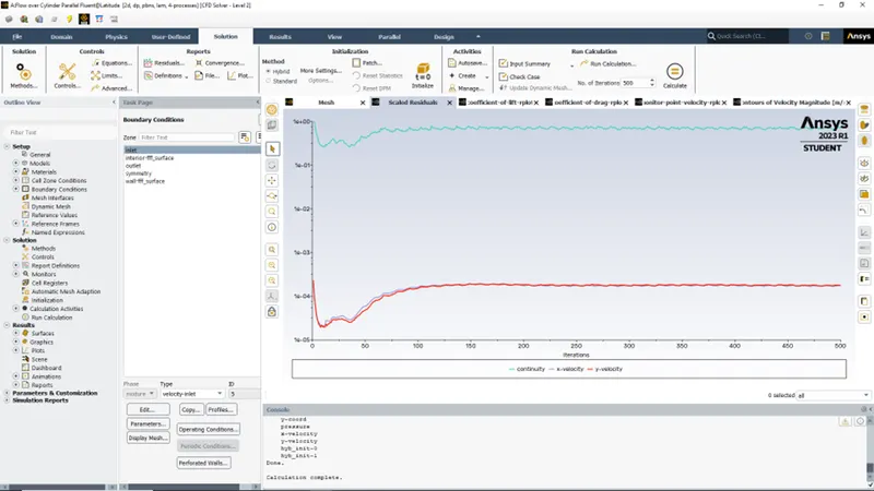
• Residual Plot

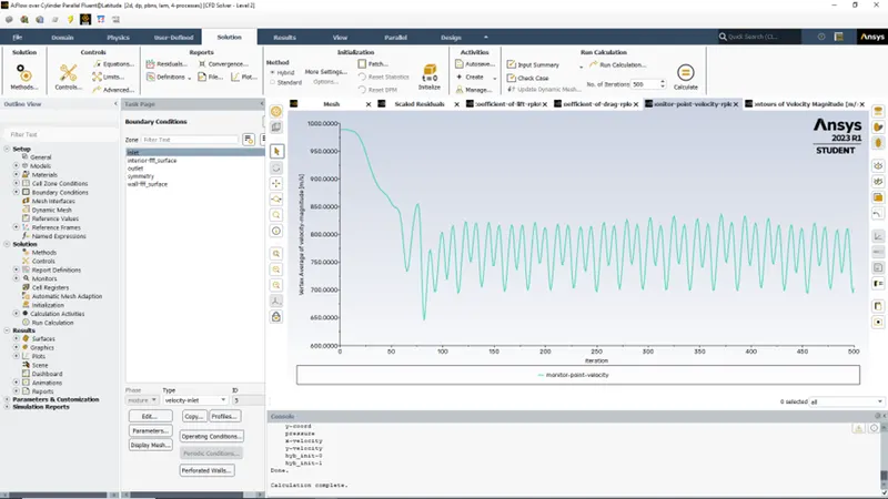
• Vertex Average of Velocity Magnitude

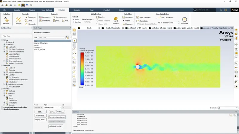
• Velocity Contour Plot

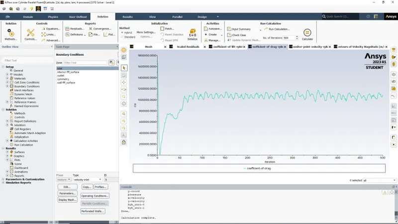
• Coefficient of Drag

• Coefficient of Lift

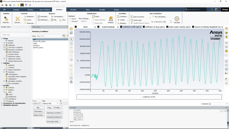
Summary of Results-

Reynold Number (Re)	Inlet Velocity (m/s)	Coefficient of drag (Cd)	Coefficient of Lift (Cl)
10	0.1	0.05436957	0.000035519044
100	1	2.1847046	0.083800725
1000	10	132.12048	77.312258
10000	100	11416.84	-4355.1536
100000	1000	1083807	767265.62

Conclusion:

1. For the Re 10, Vortex shedding & Kamran vortex street was unable to visualize for Re 10 because these phenomena don’t occur below Re 40. 
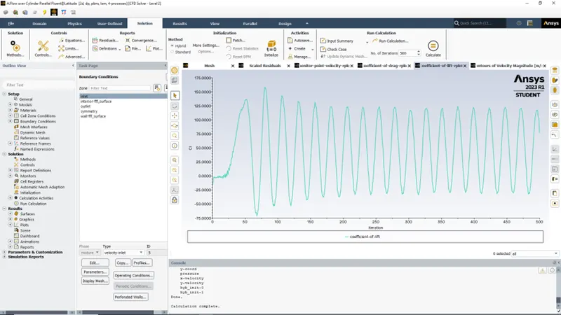
2. From the contour plot, we can see Vortex Shedding occurring in the domain for Re 100 & above. Vortex shedding can be confirmed from the Coefficient of Lift plot as well. In the Coefficient of Lift plot, we can see the oscillations in the values of it. These Osciallations confirm the occurrence of vortex shedding occurring in the domain. So, we can conclude that for Reynolds number 100 & above, there is an occurrence of Vortex Shedding for the given Geometry. 
3. The drag coefficient for the Re above 1000, is start fluctuating but periodic after one point which can be seen from the results images. So statistically, it is constant. 
4. From the results, we can conclude that the drag coefficient increases with increase in Reynolds number.