Week 1- Mixing Tee

For this challenge, we have created two versions of the mixing tee. One of them is longer than the other.

Your job is to set up steady-state simulations to compare the mixing effectiveness when hot inlet temperature is 36⁰C & the Cold inlet is at 19⁰C.

Use the k-epsilon and k-omega SST model for the first case and based on your judgment use the more suitable model for further cases. Giving the reason for choosing a suitable model is compulsory.

Aim :- To simulate the air flow thru a T-shaped pipe having two inlets and to determine mixing behaviour based on change in fluids' momentum ratio.

Theory :- T-shaped pipe has two inlets, having incoming air at different velocities and temperatures and the goal is to get the outlet air at desired temperature. T-shaped pipe is commonly used in HVAC and any other industries which inculcates working with fluid.

To begin with, the solid 3D model of pipe is loaded in Ansys Spaceclaim in order to capture the inner volume for flow simulation. Thereafter, the faces are categorised as inlet, outlet and wall.

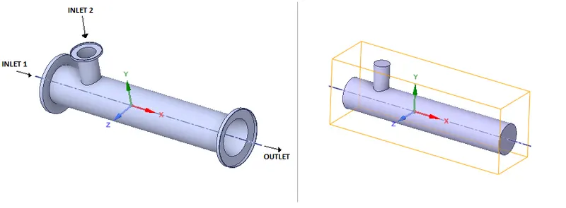
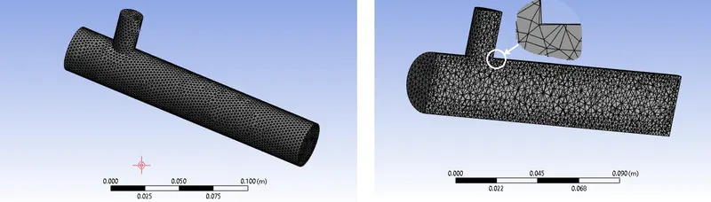
As the Finite Volume Method is more suitable for discretizing, the reason for that is the following equation obtained by applying Gauss Divergence Theorem in the General Transport Equation.

∂∂t∰(ρϕ)dV+∯(ρϕu→)dA=∯(Γ∇ϕ)dA+∰SdV">∂∂t∰(ρϕ)dV+∯(ρϕ→u)dA=∯(Γ∇ϕ)dA+∰SdV∂∂�∰(ρϕ)��+∯(ρϕ�→)��=∯(Γ∇ϕ)��+∰���

Here, the two terms are converted to the "control surfaces" from "control volume", if this is not done then the control volume can be represented via one cell centroid, on which everything will be dependent. There will not be any connections to the neighbour faces, and so the equations will get disconnected. The Finite Difference Method, having non-conservative form of equations, does not involve integration on a particular control volume, so Gauss Divergence Theorem cannot be used, so the F.D.M. will not result in conservation.

After the meshing is completed, the Inlet and Boundary conditions are setup in Ansys Fluent module. For the current analysis, "Pressure based solver" is used as the flow falls in incompressible regime where the change in density is insignificant. The solver solves the corrected values of pressure and velocity for convergence, Continuity equation, x-momentum, y-momentum, z-momentum equation and since the temperature is involves, the Energy Equation is solved as well.

Secondly, two turbulence models are selected for the analysis, namely k-epsilon Realizable and k-omega SST. Also, as a part of working fluid, air is selected at standard conditions of pressure and kinematic viscosity.

With momentum ratio of 2 (ratio of Velocity of cold to that of hot fluid) inlet conditions are set as :-

Face	Type	Value
Inlet 1 (hot)	Velocity inlet	vh=3m/s T = 36°C
Inlet 2 (cold)	Velocity inlet	vc=6m/s T = 19°C
Outlet	Pressure outlet	p = 1 atm
Wall shear	No slip	Surface velocity = 0

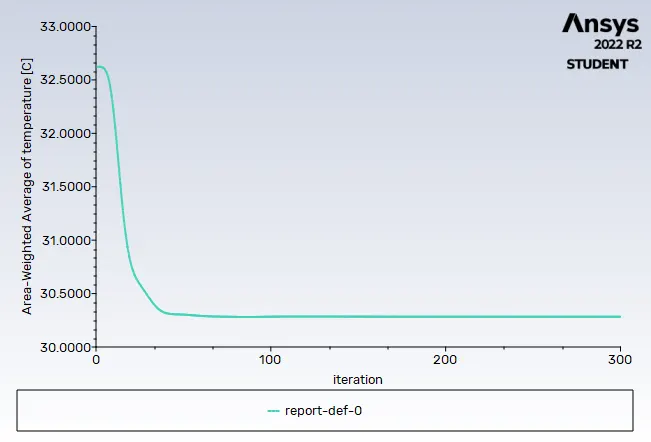
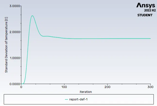
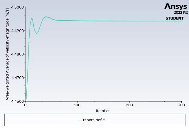
Nextly to observe the variation in Velocity and Temperature profile, reports for Average temperature and velocity throughout pipe, Standard deviation in temperature and Residuals (which are functions used in PDEs for making approximations and are not evaluated as 0) are defined. Before running calculation, the 'Hybrid' initialization is chosen which involves Potential flow solver to compute values for velocity and pressure and the calculation is run for 300 iterations.

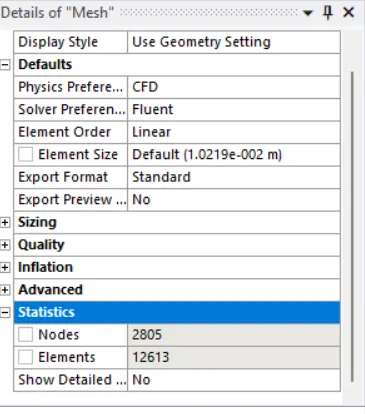
Results :-

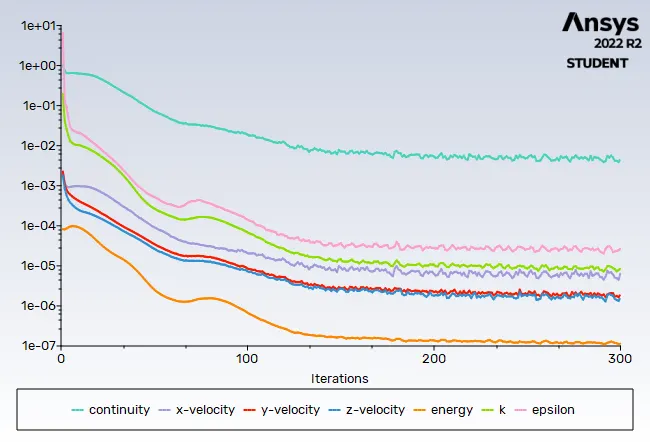
Plots with k-epsilon Realizable model for short pipe and Momentum ratio 2:

Plots with k-omega SST model for short pipe and Momentum ratio 2:

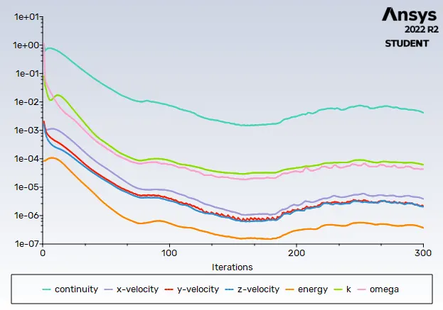
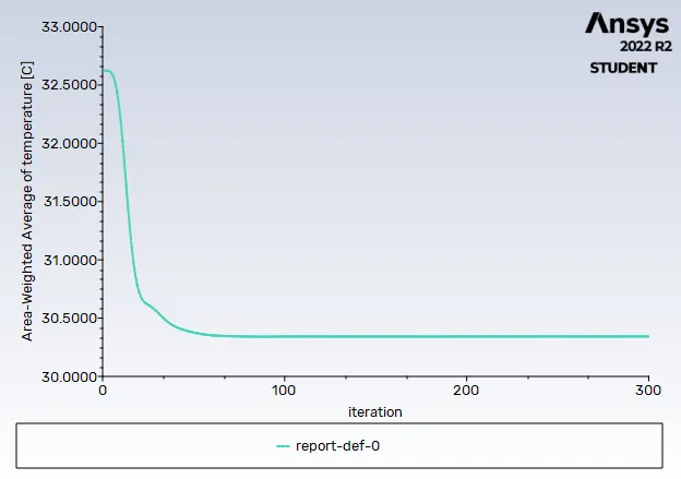
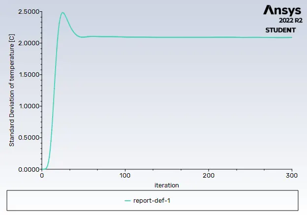
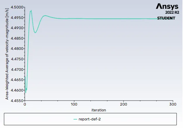
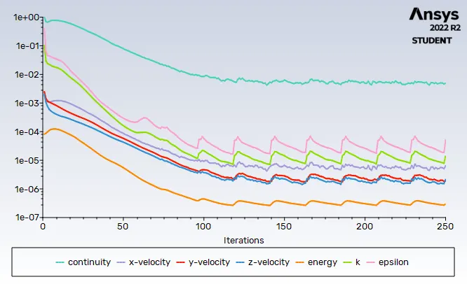
As seen for k-epsilon model's plots, the iterations for the equations start to converge after around 130, whilst, for the k-omega model, more iterations will be required for the solutions to converge.

Similary, following is noted from above plots:

	Residual convergence after iterations	Area weighted avg. Temperature	Std. deviation of Temperature	Area weighted avg. of velocity
k-epsilon	130	30.48	1.8	4.4950
k-omega	more than 300	30.48	2.1	4.4950

1]. Flow in a Short pipe

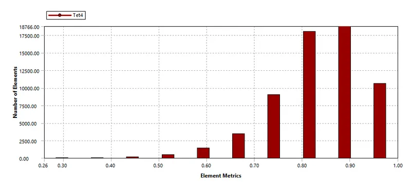
Case 1.a : Short pipe with Momentum ratio 2, k-epsilon model and Mesh quality 0.0025

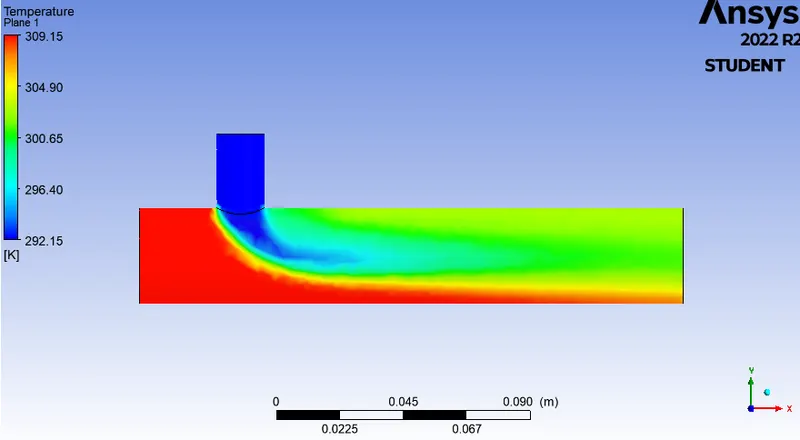
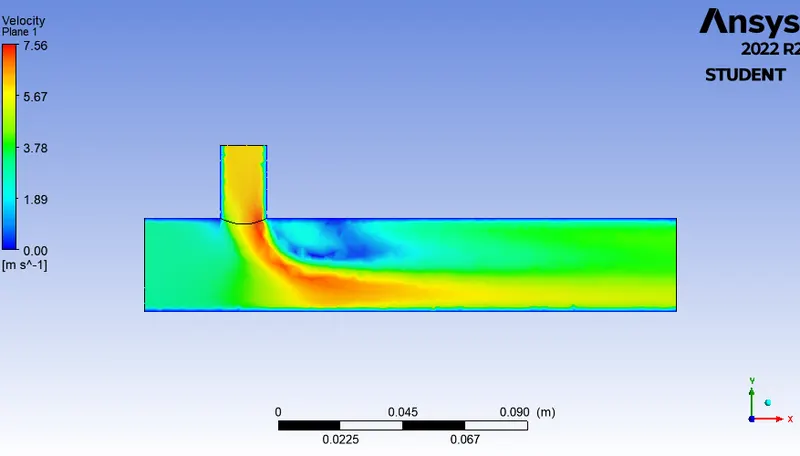
Case 1.b : Short pipe with Momentum ratio 4, k-epsilon model and Mesh quality 0.0025

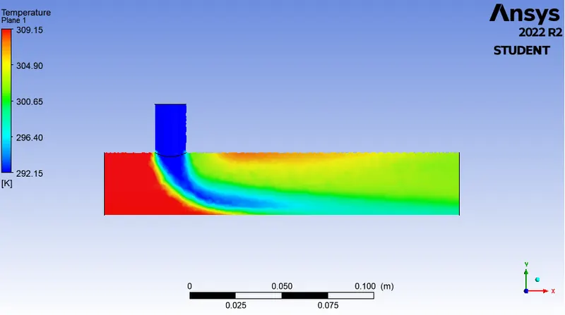
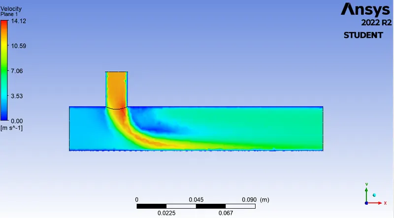
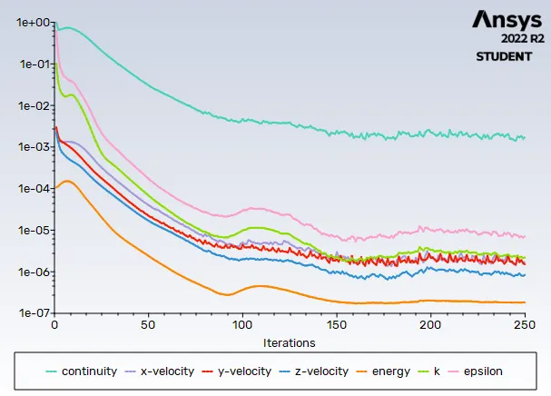
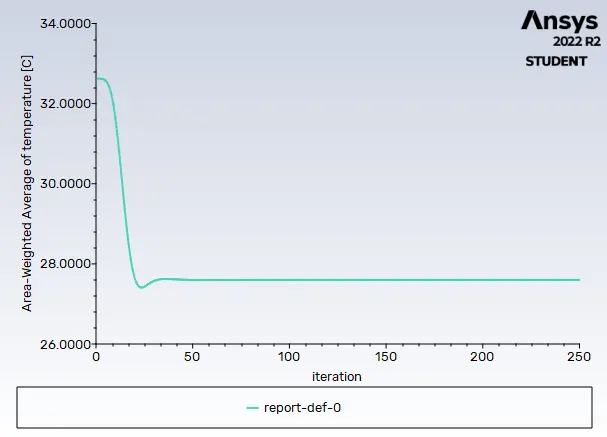
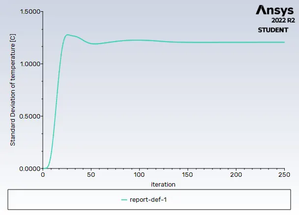
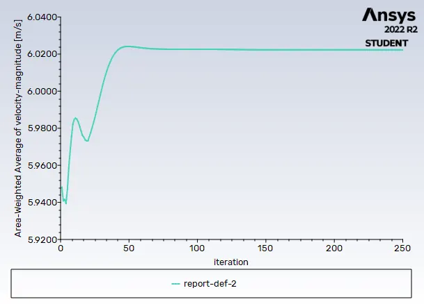
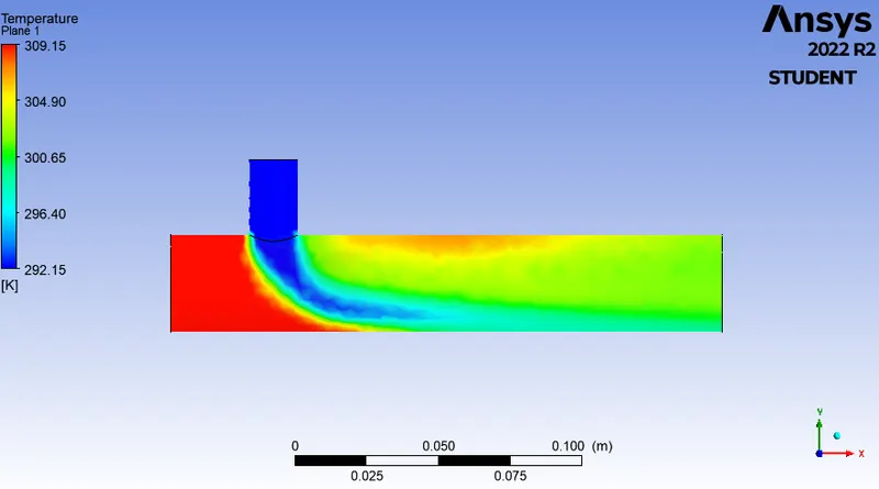
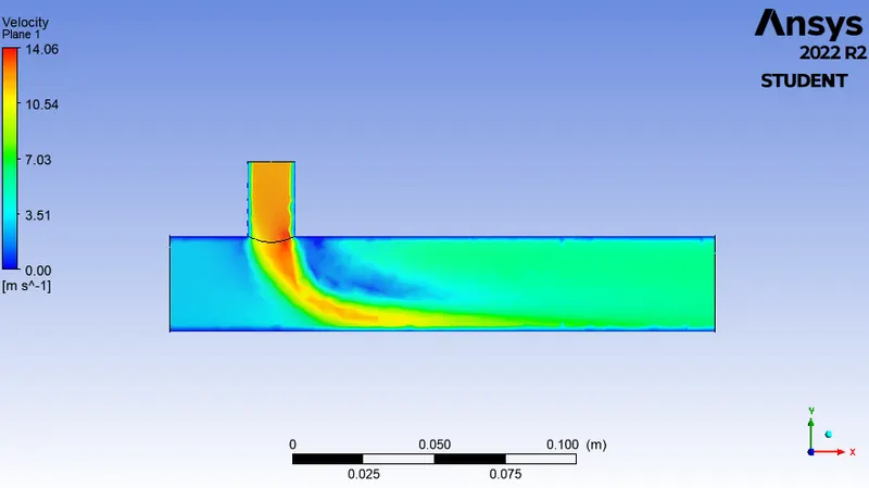
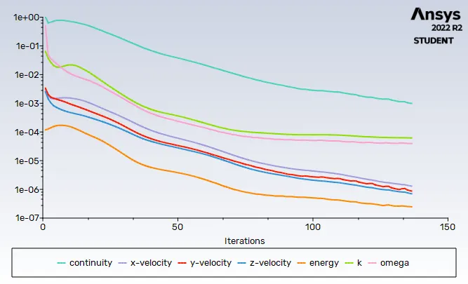
Case 1.c : Short pipe with Momentum ratio 4, k-omega model and Mesh quality 0.003

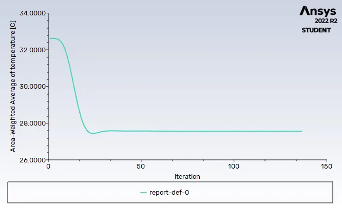
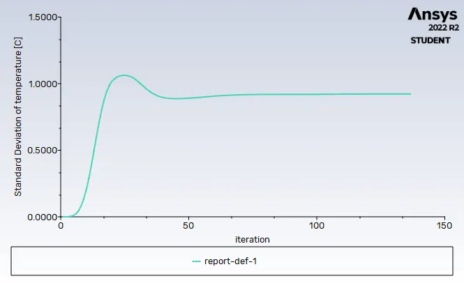
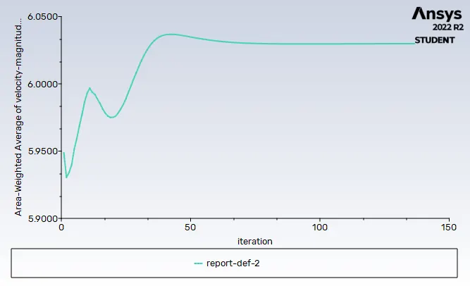
Results for Short pipe simulation :-

Case	Cells	Model	Iterations	Outlet Temperature
1.a Momentum ratio 2	18766	k-epsilon	approx. 300	30.35 °C
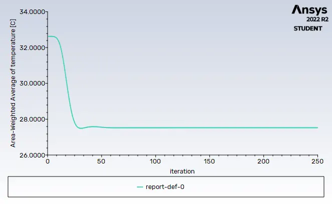
1.b Momentum ratio 4	18766	k-epsilon	around 250	27.5 °C
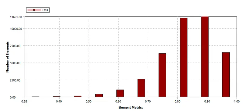
1.c Momentum ratio 4	11691	k-omega	around 140	27.5 °C

2]. Flow in a Long pipe

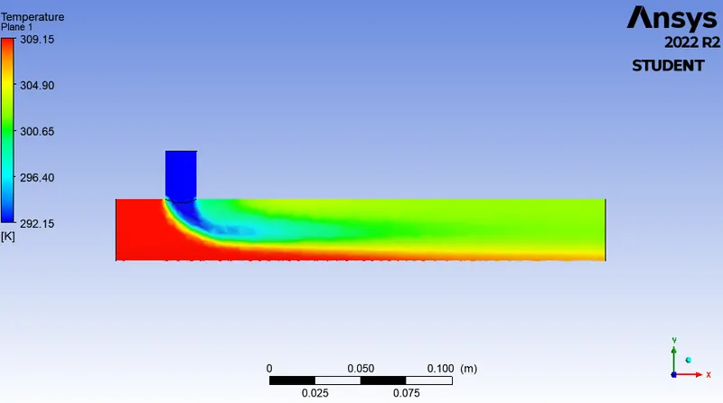
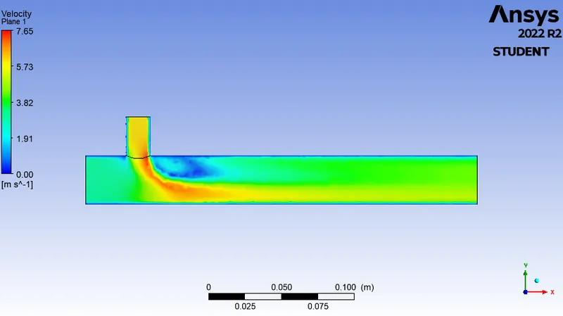
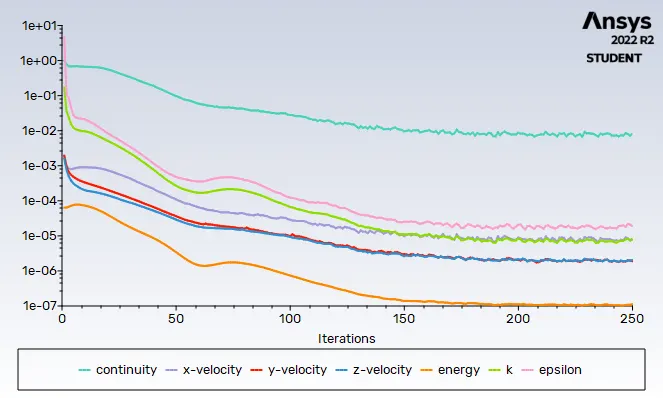
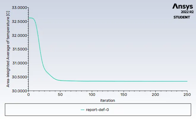
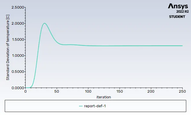
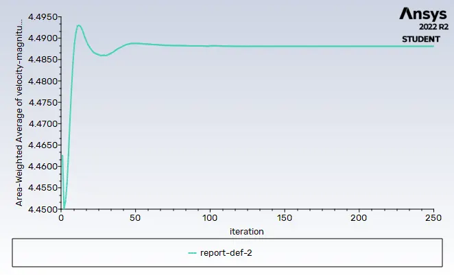
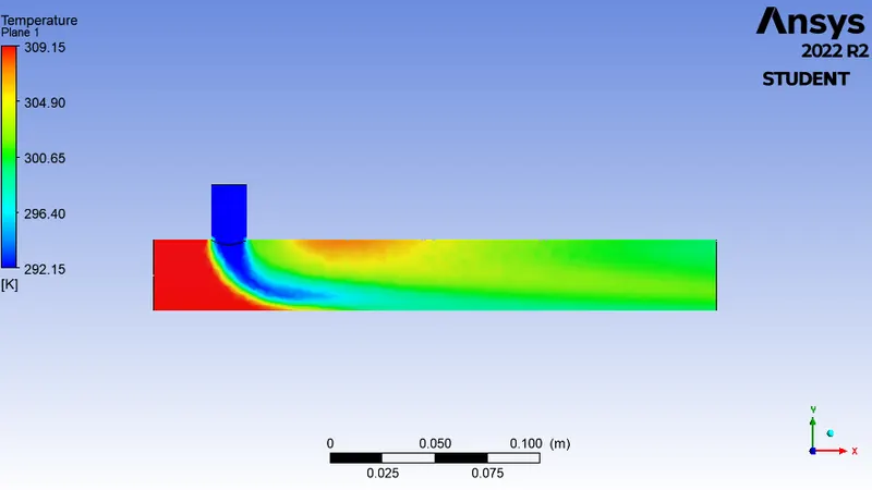
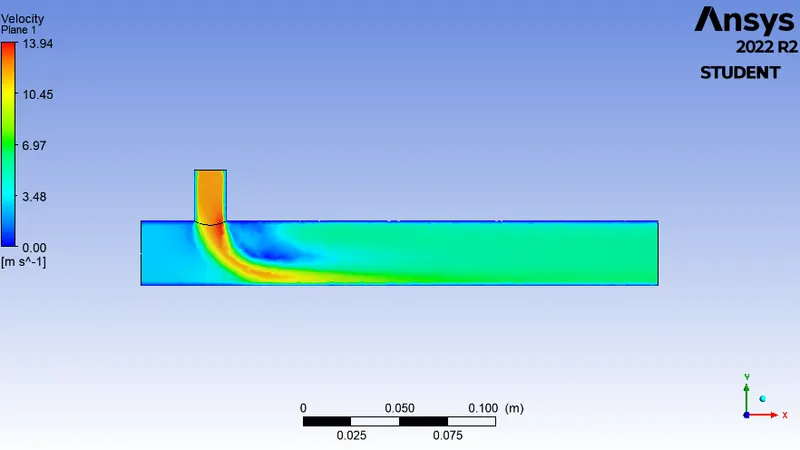
Case 2.a : Long pipe with Momentum ratio 2, k-epsilon model and Mesh quality 0.0025

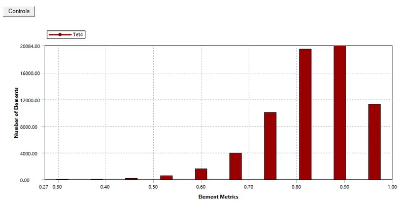
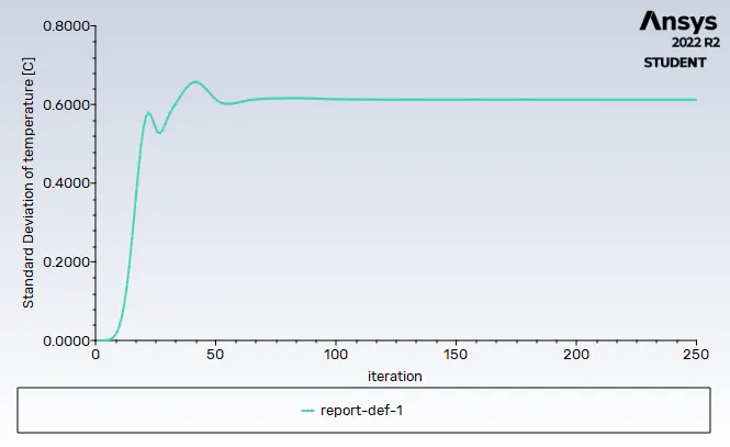
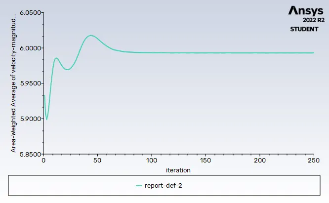
Case 2.b : Long pipe with Momentum ratio 4, k-epsilon model and Mesh quality 0.0025

Case 2.c : Long pipe with Momentum ratio 2, k-omega model and Mesh quality 0.0025

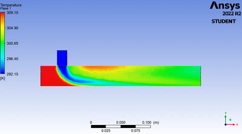
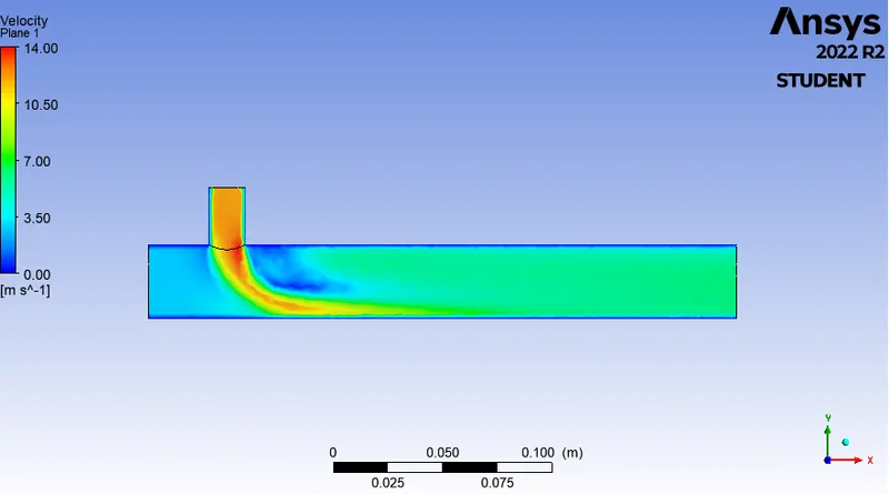
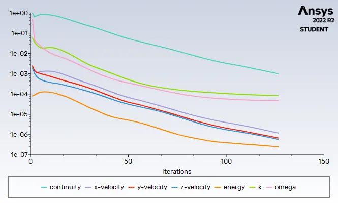
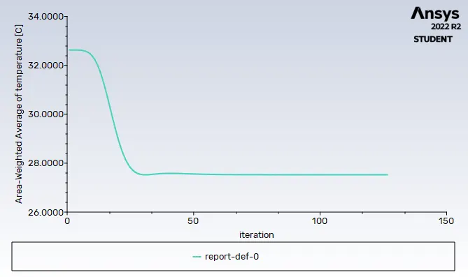
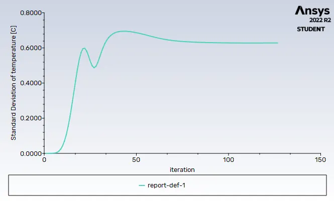
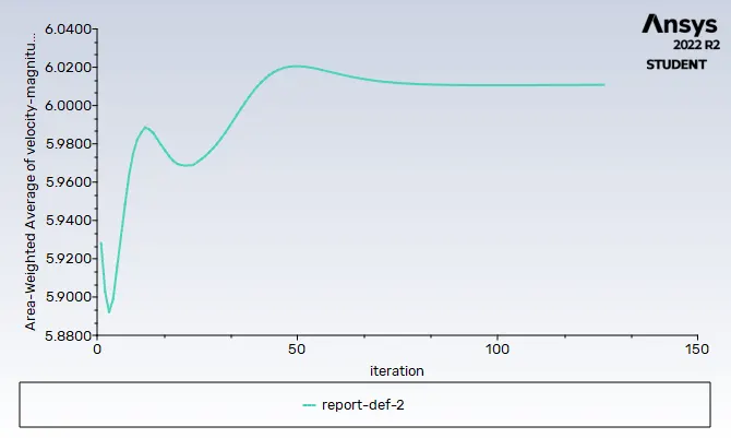
Results for Long pipe simulation :-

Case	Cells	Model	Iterations	Outlet Temperature
2.a Momentum ratio 2	20084	k-epsilon	around 250	30.40 °C
2.b Momentum ratio 4	20084	k-epsilon	more than 250	27.5 °C
2.c Momentum ratio 4	20084	k-omega	around 135	27.5 °C

Conclusion :-

In order to get mixing efficiently, flow with higher Momentum ratio is more desirable. In first case, i.e. for short pipe, the outlet temperature is more when the cold inlet has fluid with high velocity and vice versa. Secondly, the iterations depends on total cells as governing equations are solved fora each cell, however with same Momentum ratio and with reduced number of cells, outlet temperature does not differ a lot.

For the long pipe, with k-epsilon model, the iterations are slowly converging to a value as seen in Case 2.b, still there are intermittent fluctuations for getting to a solution, while using the k-omega model, which is more suitable for capturing near wall effects, convergence is resulted smoothly with less iterations. Standard deviation of temperature is higher in case of flow with higher Momentum ratio.