Performing CFD analysis of a mixing tee

Aim: Performing CFD analysis of a mixing tee.

Objective:

• Understand the concept of a mixing tee, its use and simulation.
• Understand and evaluate the problem statement and the required CFD approach to solve the problem.
• Judge the suitability of a turbulence model for the given problem (here, k-epsilon and k-omega SST)

Introduction:

A mixing tee is a pipe fitting, wherein two fluid streams form a mixture and the entry of the flow of these fluids is perpendicular to each other. This mixing takes place for mass and heat transfer between one or more streams, fluids, components and phase and thereby form a combined stream. This configuration is widely used in domestic or commercial plumbing, petrochemical industry and HVAC industry for obtaining a desired mixture.

In this case, a comparative analysis of two different mixing tee configurations is done to obtain the mixing effectiveness for given boundary conditions (the inlet temperatures and velocity).

Workflow:

1. Preparing the geometry, (geometry clean-up)
2. Generate mesh for the geometry
3. Setting up the solver
4. Setting up the solution monitors
5. Post-processing to observe the results

Ansys Fluent:

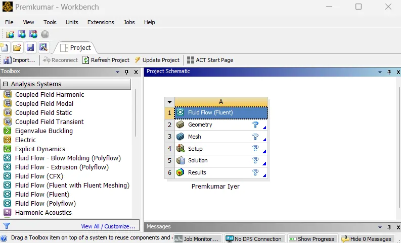
In the Ansys workbench project window, Fluid Flow (Fluent) is dropped into the workspace.

Preparing the geometry (CAD Cleanup):

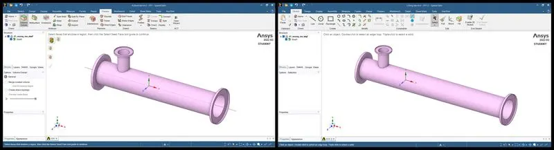
This geometry was provided to us for performing the simulation. The geometry is imported to Ansys SpaceClaim (left: short tee, right long tee)

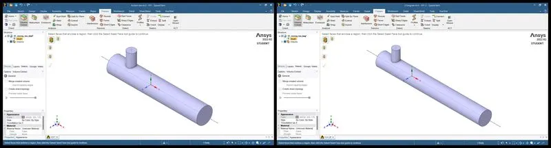
Since, we are interested in the flow occuring in the "piped" domain of the geometry, we cleanup the geometry as follows. Using the volume extract feature in the "Prepare" tab of SpaceClaim, the flow domain is defined. The edges of inlet and outlet were selected to do so. Now we have the volume region and the outer body is separated as a shell. This shell is inactivated for visibility (it is kept hidden) and suppressed for physics. Thus, we obtain the volume extract as shown below.

Generating mesh:

Meshing is the process, wherein the geometry is divided into smaller parts which are known as elements, so that the iterative solver can solve the governing equations across the domain. In the meshing utility, a medium mesh was provided for the given geometries. The element size is 2mm. The mesh metrics too were observed for the generated mesh.

For short tee:

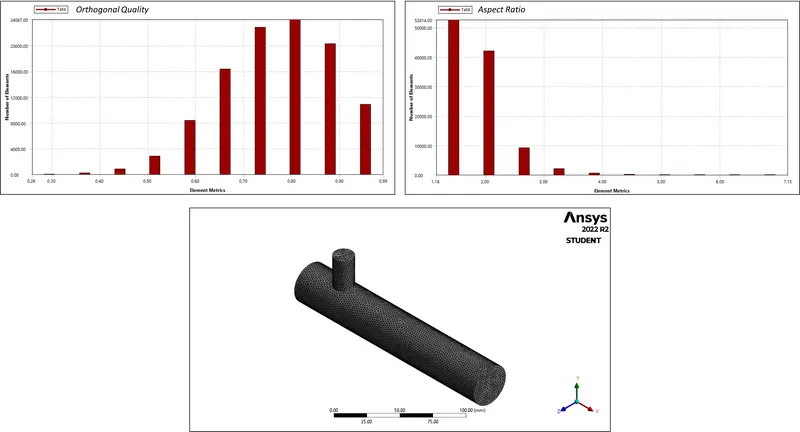
For long tee:

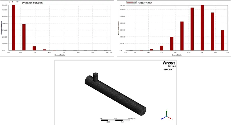
For implementing the boundary conditions, the "boundaries" must be clearly defined. To do so, the mesh utility itself has a tool; named selections. By selecting the respective faces and surfaces, the inlet for hot and cold fluids, the outlet and the wall as well was defined.

Setting up the solver:

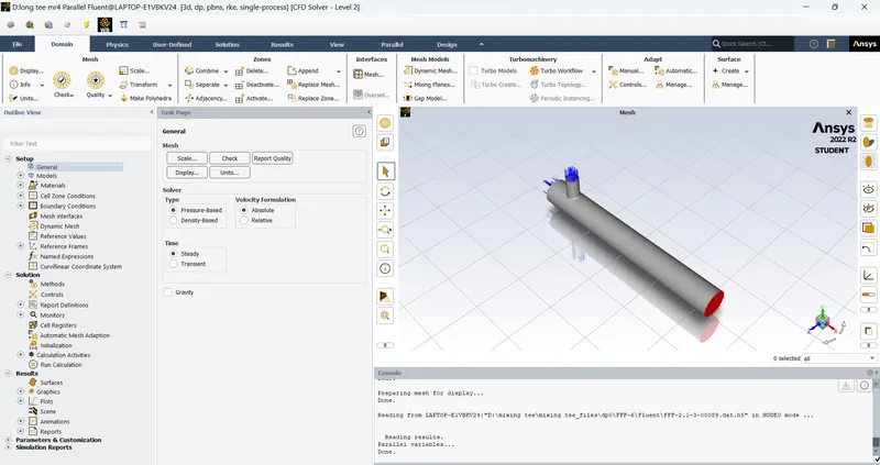
The important part of the CFD simulation, we set up the solver for obtaining the solution. Firstly, the units of important parameters is checked (e.g. length in meters, temperature in deg Celsius). In the models tab, energy equation is switched ON (since it is a heat transfer problem). Further, as the problem is based on turbulence flow, the k-epsilon model (realizable with standard wall functions) is used and the reasons are discussed in the conclusion. The fluid material here is air, which is the default material present in Fluent and hence was left unchanged. Later, the boundary conditions are provided; inlet velocities and temperatures at cold & hot inlet and outlet of the tee is left untouched. The hot inlet velocity is kept constant (3m/s) and the cold inlet velocity is varied as per the momentum ratio.

The momentum ratio (M.R.) here is defined as:

`M.R. = (Velocity at cold i n l e t)/(Velocity at hot i n l e t)`

Case	Momentum Ratio	Hot Inlet		Cold Inlet
		Velocity	Temperature	Velocity	Temperature
Short Tee	2	3	36℃	6	19℃
	4			12
Long Tee	2			6
	4			12

The pressure-velocity coupling is set to coupled and the energy, turbulence, momentum and pressure are set to second order. In order to capture some important insights from the outlet, report definitions are created; namely, area-weighted-average of the temperature at outlet and the standard deviation of the outlet temperature. Their respective plots along with the residual plot is saved after the solution converges. Hybrid initialization is used to initiate the solver, thereafter, a certain number of iterations is entered (say, 200) and calculations start.

Post-processing (Results):

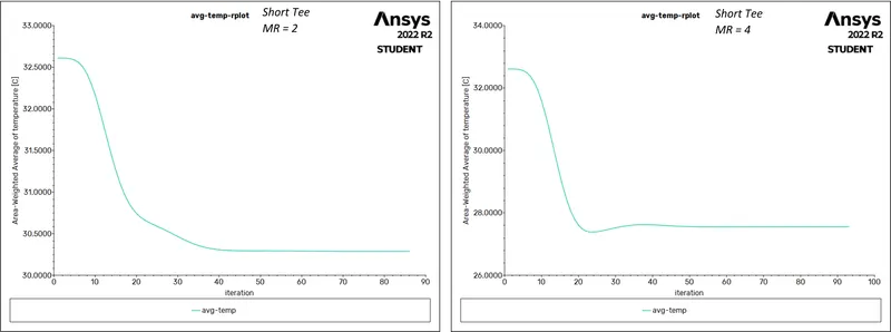
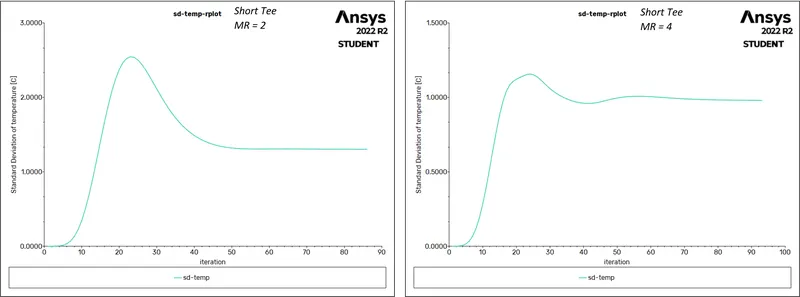
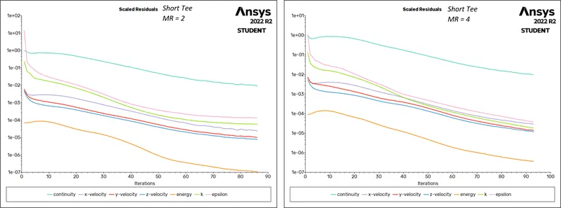
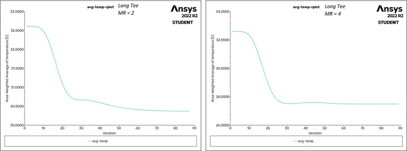
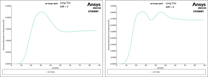
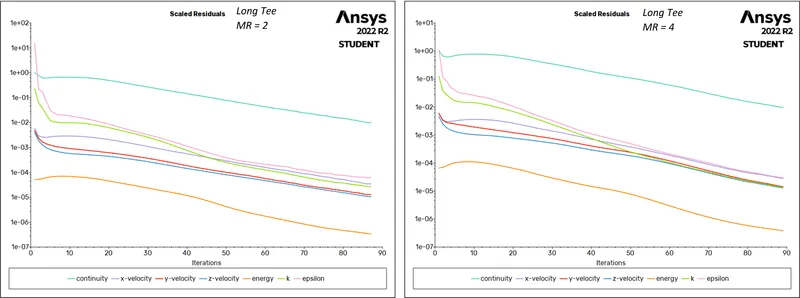
The above are the plots for area weighted average temperature at outlet, standard deviation of temperature at outlet and residuals respectively.

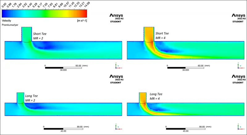
The velocity countours

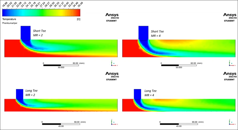
The temperature contours

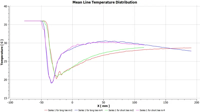
Temperature distribution along the centreline of the mixing tee

Case	Mesh Size	Outlet Temperature (℃)		No. of Iterations
		Area Weighted Average	Standard Deviation
Short Tee	106539	30.28746	1.3023560	86
		27.55250	0.9794594	93
Long Tee	140990	30.36982	1.4343100	87
		27.49169	0.6796126	89

Conclusion(s):

• Hence, a brief study of effect of mixing length and momentum of mixing fluids on the mixture obtained at the outlet was done successfully.
• As far as turbulent models are concerned, k-epsilon and k-omega are two profound solvers. To choose between them, an important question needs to be answered, what is the region of importance, the bulk flow (or free flow) of the fluid or the flow happening near the walls (hence, velocity and pressure gradients resulting this)?
• The k-epsilon model is a resource-friendly and pretty accurate two equation based solver which is generally used for external flows. However, there are limitations of its application where there are adverse pressure changes happening (e.g. no slip walls, or in the viscous sub-layers). However, the realizable k-epsilon improvises this by taking into account the effects of mean flow distortion on the turbulent energy dissipation.
• The k-omega model, on the other hand, is more suitable for flows near the walls (or capturing near wall interactions). The main problems associated with this model is that, the flow separation and free flows are overpredicted and the solutions obtained are comparatively difficult to converge.
• In this case, we are intereseted in the interaction between the two flow streams, mixing into each other (thus, a free flow problem), the k-epsilon model became a de facto choice.
• In the cases studied here, it was evident that with an increase in momentum ratio, the mixing is quite vigorous (as seen in the temperature contours) as the turbulent nature of the flow regimes is enhanced (as seen in the velocity contours). Also, in case of lower momentum ratio, it was observed that some hot fluid is expelled without even getting mixed.
• Moreover, it was observed that with an increase in the mixing length, the mixture attains more uniformity in terms of the temperature of mixed fluid at the outlet. That is the mixture settles after the vigorous mixing, and thus the uniformity is experienced.
• Hence, it can be concluded that turbulence is an essential component of mixing, and thus, while design of such fittings (a mixing tee per se), care needs to taken regarding the uniformity of mixture which is highly dependent on the incoming streams interact and how the resultant mixture is allowed to settle.

Reference(s):

• Introduction to GUI based CFD using Ansys Fluent - course provided by Skill Lync
• ANSYS Inc.
• Supporting Material: Ansys Fluent User Guide; Modelling Turbulence
• Supporting Material: Turbulence models: Spalart-Allmaras, k- Epsilon and k-Omega
• Supporting Material: Choosing the Right Turbulence Model for Your CFD Simulation

Materials: The workbench file, plots, contours can be accessed here