Week 1- Mixing Tee

Week 1 Challenge - Mixing Tee: Detailed Report

Objective:-

Steady state simulation of mixing tee and compare the mixing effeciency when hot inlet temperature is 36oC36oC and cold inlet temperature is 19oC19oC using ANSYS Fluent.

Case 1 (a):

• Short mixing tee with a hot inlet velocity of 3m/s.
• Momentum ratio of 2,K-epsilon Model

PROCEDURE:

1. Geometry Importing and Volume Extraction:

• First open Ansys Workbench and click on Fluid Flow (Fluent) and drag it to the GUI screen.
• Then double click on geometry to navigate to Ansys Spaceclaim. Here open the required file.
• The short mixing tee geometry will look as below:

The long mixing tee geometry is as follows:

• Since the analysis is only done for the wet volume hence only that is volume is extracted. For this select volume extract -> select edges and select the edges where fluid has contact with the body. The geometry with dimensions will look as below:

Short tee model:

• Now after the wet volume is extracted the dry volume which is the shell is not to be included for the simulation. For which Suppress for Physics option is selected for the shell.

2. Meshing:

• Now the geometry is meshed using the mesh option available in the workbench. Here tetrahedral mesh type is used.
• The mesh size is 4mm i.e. 4e-003 m and the meshed model is as below:

meshed model for short tee geometry:

• The faces of the geometry are given their respctive names as below:

3. Solving:

• Now the meshed component is solved using ansys fluent for which double click on setup option in workbech GUI to navigate to Fluent.
• Here the boundary conditions are set and solutions are obtained.

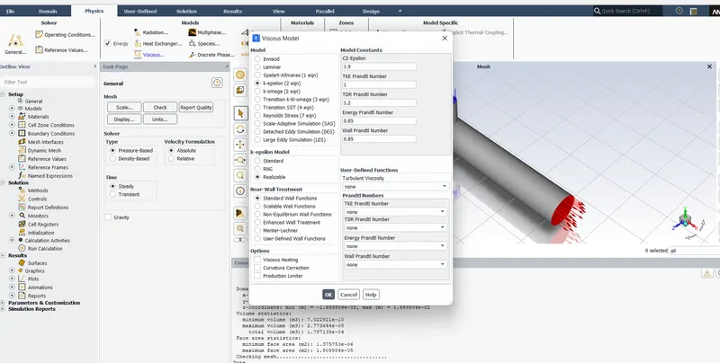
Given K-Epsilon model and enegy equation also on.

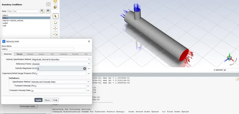
giving cold inlet velocity as 6m/s.

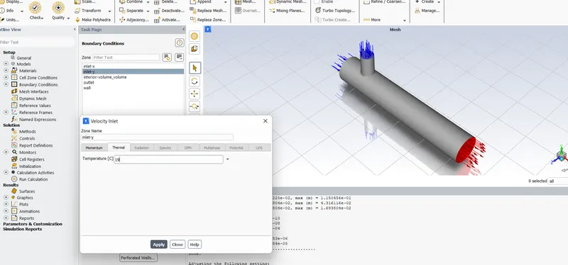
Giving cold inlet temperature as 19 deg celcius.

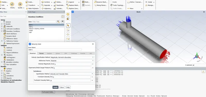
Giving hot onlet velocity as 3m/s.

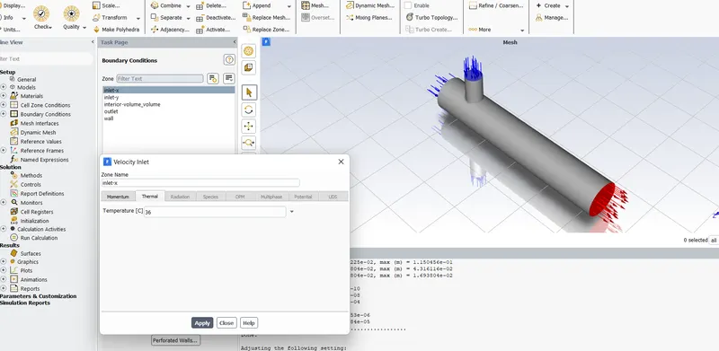
Giving hot inlet temperature as 36 deg. cel.

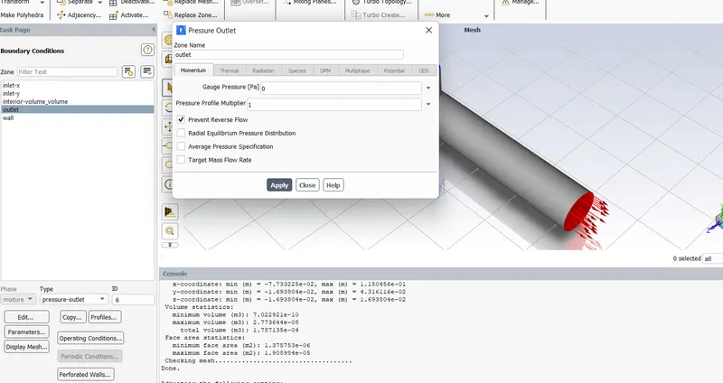
Giving pressure outlet as 0 gauge pressure ie 1 atm pressure.

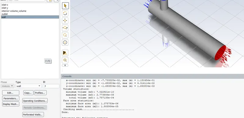
For wall it is given as wall boundary conditions.

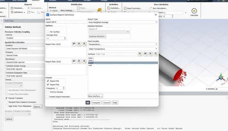
Giving area-weighted average of temeperature at outlet.

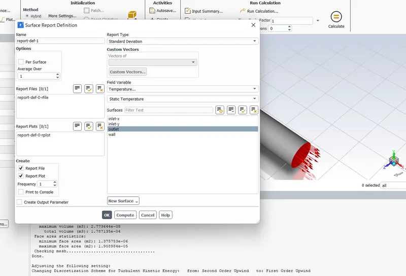
Taking standard deviation of temeprature also at outlet.

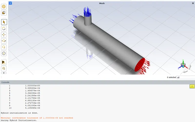
Hybrid initialization done.

RESULTS AND DISCUSSIONS:

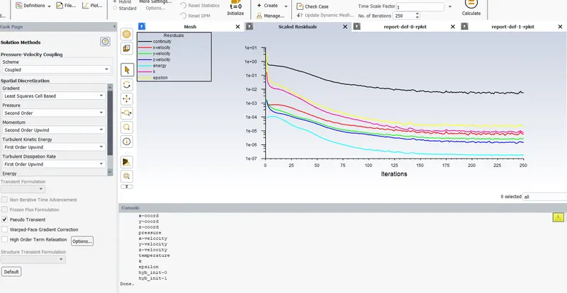
Given total no of iterations as 250 and it is showing that al residuals converged.

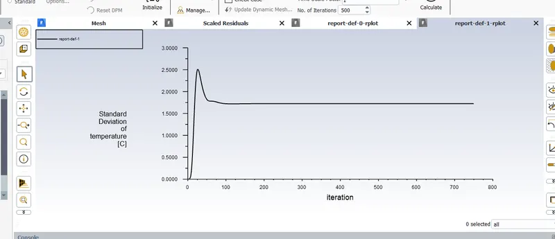
Showing standard deviation of temeperature at outlet and it showing aroung as 1.7 means there is no much difference in temeperature at outlet from the mean value.

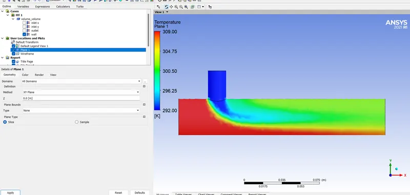
It is showing that the temperature distribution along the lenghth of mixing tee.

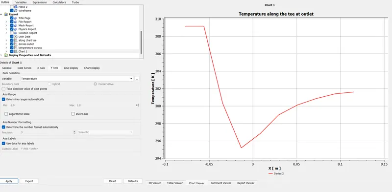
Plot of temperature distribution along the tee

From this temeperature contour and plot we can understand that, the hot fluid is coming through the bottom inlet and cold fluid is coming through the top inlet and finally they mix together and we will get a temperature of combination of these two flows at the outlet.

At the outlet we get a temeperature near 300k (27deg cel).

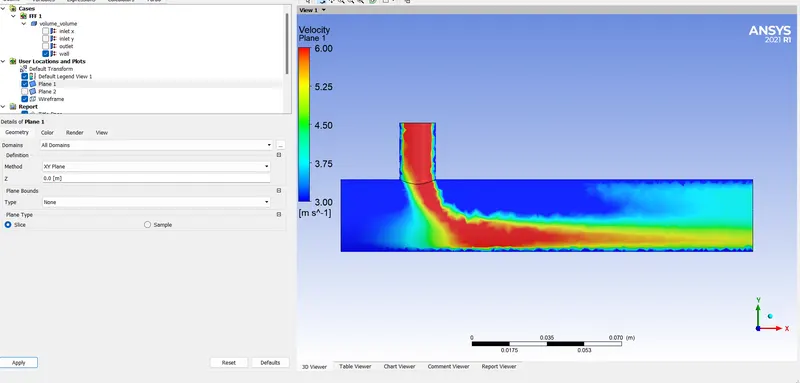
It is showing that the velocity distribution along the lenghth of mixing tee.

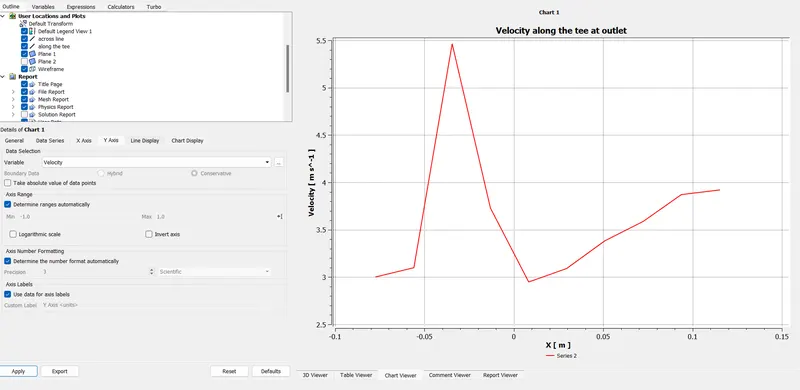
Plot of velocity distribution along the tee

From this velocity contour and plot we can understand that, the hot inlet velocity is 3m/s and cold inlet velocity is 6m/s and therefore the momentum ratio is 2.

Here cold inlet velocity is 2 times than hot inlet velocity and as a result cold jet is impinging and mixing with hot jet at the tee junction and some turbulence occuring at the mixing junction and gradually it is reducing as flow moves forward and at outlet we will get a velocity around 3.75m/s.Maximum velocity is at near the mixing junction.

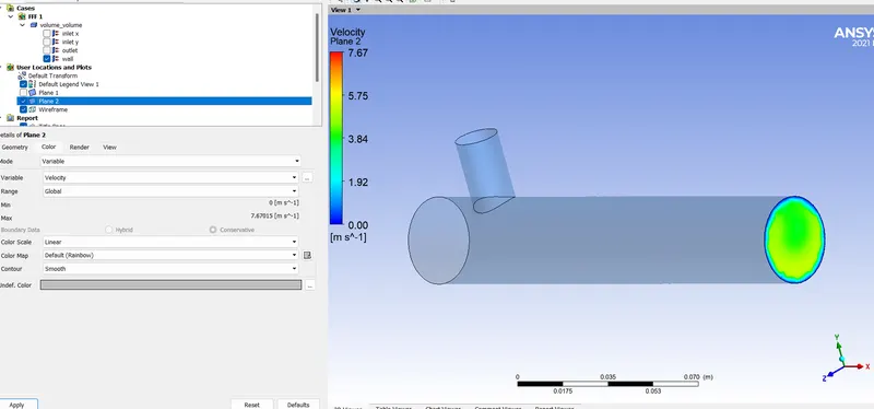
It is showing the velocity distribution at oulet and across the pipe.

From this figure we can understand that due to the boundary layer effect velocity of flow is very less near to the wall and velocity is gradually increasing towars the centre of pipe.At the centre velocity of flow is around 3.87m/s.

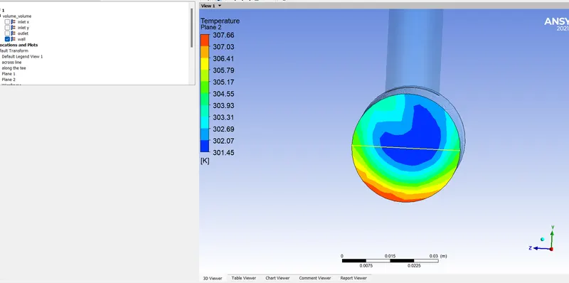
This figure shows the temperature ditribution across the pipe at outlet.

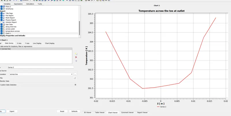
Plot of temperature distribution across the tee at outlet.

From the above plot and contour we can understand that temperature is less at the centre and and maximum at the bottom side.This may be due to the position of cold inlet is at the top of tee.

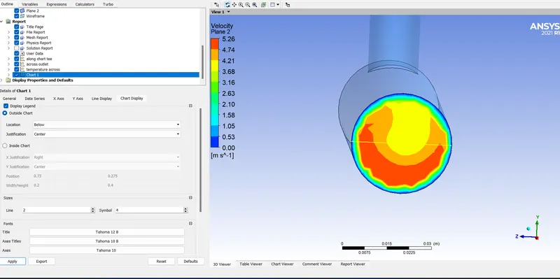
Contour of velocity across the tee at outlet.

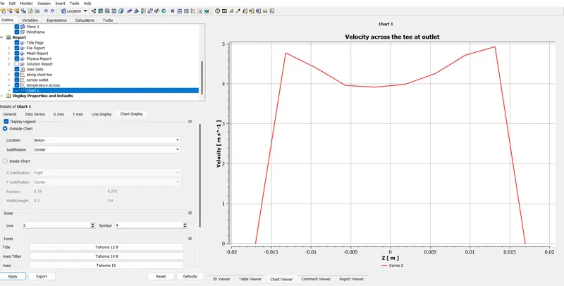
Plot of velocity across the tee at outlet.

From the above contour and plot we can understand that velocity is minimum near the walls due to boundary layer effects and gradually increases towards centre.

Case 1 (b):

• Short mixing tee with a hot inlet velocity of 3m/s.
• Momentum ratio of 4 , K-epsilon model.

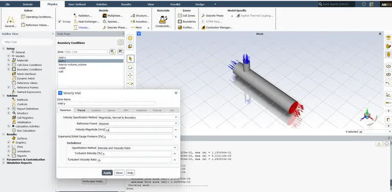
Given cold inlet velocity as 12m/s.

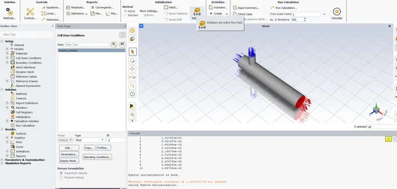
Hybrid initialization done.

RESULTS AND DISCUSSIONS:

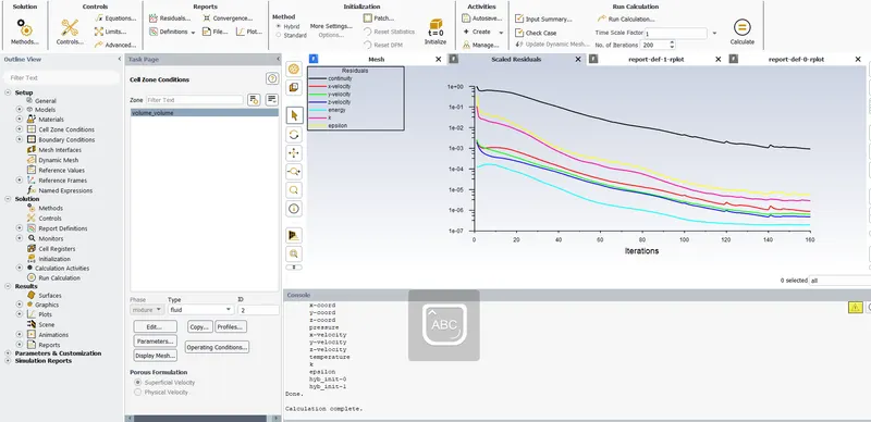
The above figure shows the residuals.

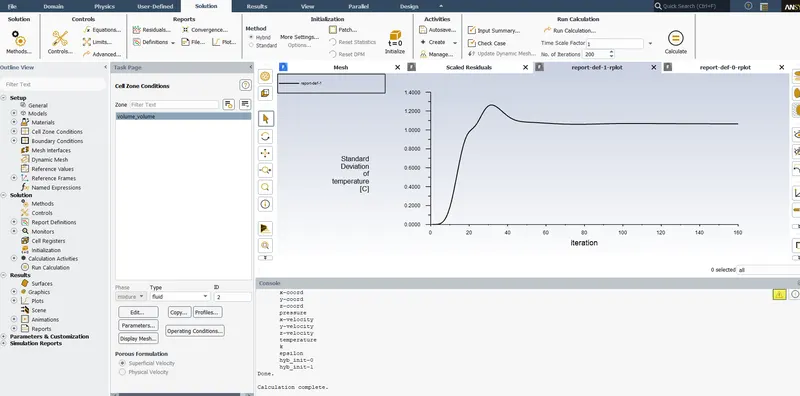
Above figure shows standard deviation of temperature.

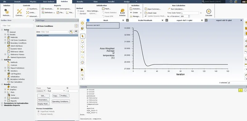
Above figure shows the area weighted average of temeprature.

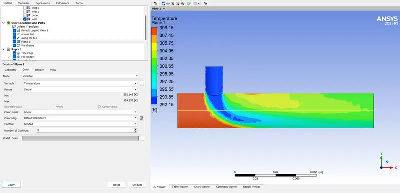
Above figure shows the contour of temperature distribution along the tee.

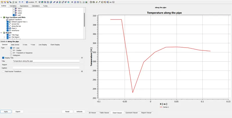
Above plot shows the contour of temperature distribution along the tee.

From the above contour and plot we can understand about the temperature distribution along the tee.Here wecan see that temeprature is maximum at horizontal inlet side and which is reducing while mixing with the cold inlet at the tee junction,so temeprature is suddently drops at the tee jucntion and then gradually increasing after that , finally reach a temeperature between hot and cold inlets.

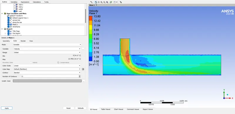
Above figure shows the contour of velocity distribution along the tee.

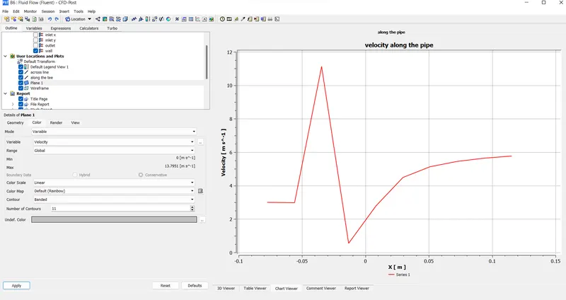
Above plot shows the contour of velocity distribution along the tee.

From the above contour and plot we can understand about the velocity distribution along the tee.Here we can see that velocity is maximum near to tee jucntion and that is for cold jet and which is reducing toward the wall due to the boundary layer effects.Due to the sudden mixing of cold jet with hot jet after reaching to a maximum velocity the velocity of jet suddently came down and then increases gradually and finally reach a velocity between cold and hot jets.

Case 1 (c):

• Short mixing tee with a hot inlet velocity of 3m/s.
• Momentum ratio of 4 , K-omega model.

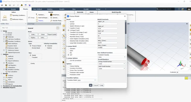
Setting K-Omega turbulence model.

RESULTS AND DISCUSSIONS:

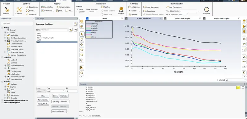
The above figure shows the residuals.

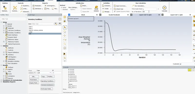
The above figure shows the area weighted average of temperature at the outlet and here the mean temeperature at outlet is 27.5 deg cel.

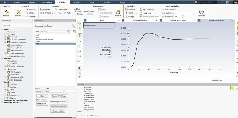
The above figure shows the standard deviation of temperature at the outlet.

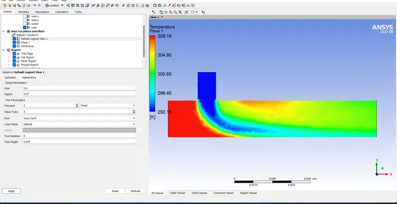
Above figure shows the contour of temperature distribution along the tee.

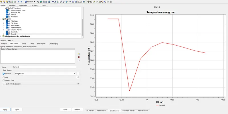
Above figure shows the plot of temperature distribution along the tee.

From the above two figures we can understand about the temperature distribution along the tee. It shows that the maximum temperature is around 309 K and minimum temperature is around 292.15K. Due to the mixing of cold jet with hot jet at the tee junction temeperature of flow is getting down very fast and then gradually increasing as flow move forward and when it reaches at outlet the temperature is around 301K.

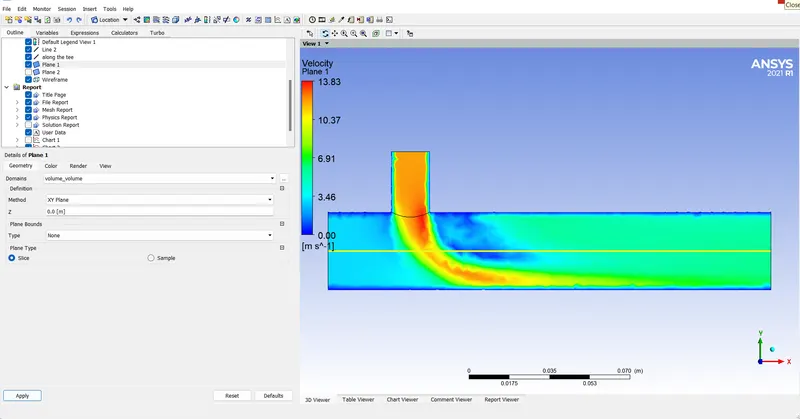
Above figure shows the contour of velocity distribution along the tee

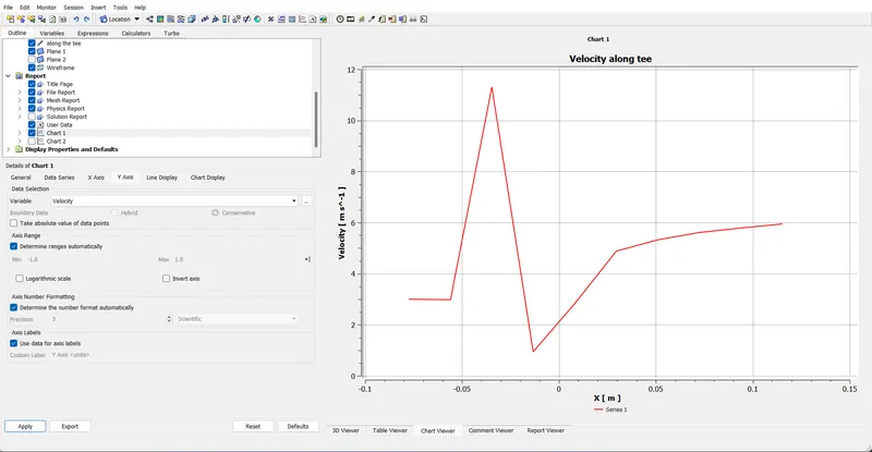
Above figure shows the plot of velocity distribution along the tee

From the above two figures we can understand about the velocity distribution along the tee.It shows that the maximum velocity is around 12m/s and minimum velocity is present near to the walls due to no-slip condition. At the tee junction, the velocity is suddently increasing due to the mixingnthen it become suddently decreasing due to the mixing effect and then gradually increasing.

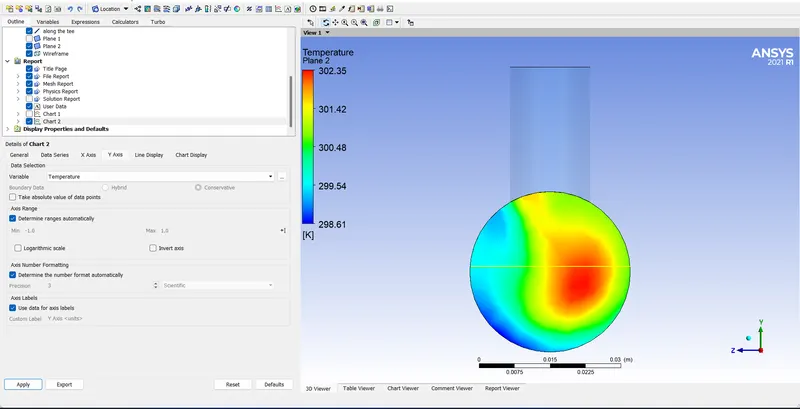
Above figure shows the contour of temperature distribution across the tee at outlet.

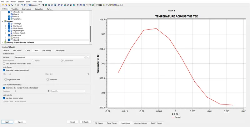
Above figure shows the plot of temperature distribution across the tee at outlet

From the above two figures we can understand about the temperature distribution across the tee.It shows that the maximum temperature is around 302.3K and minimum temperature is around 299.5K and which is present at the left side of the pipe.To the middle portion, temperature is increasing reaches a maximum value then slowly decreasing.

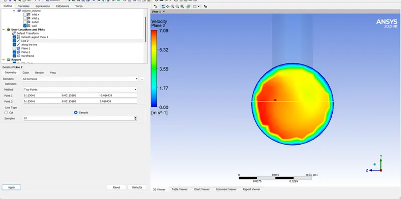
Above figure shows the contour of velocity distribution across the tee at outlet

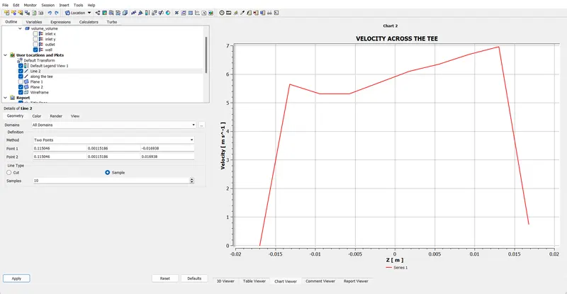
Above figure shows the plot of velocity distribution across the tee at outlet.

From the above two figures we can understand about the velocity distribution across the tee.It shows that the maximum velocity is around 7m/s and minimum velocity is present near to the walls due to no-slip condition.

Note: As per the study, we can't see much difference between K-Epsilon and K-Omega turbulence model.But K-epsilon model is more suitble for low Reynolds number problems and for the second case I am using K-Epsilon model.

Case 2 (a):

• Long mixing tee with a hot inlet velocity of 3m/s.
• Momentum ratio of 2, K-Epsilon.

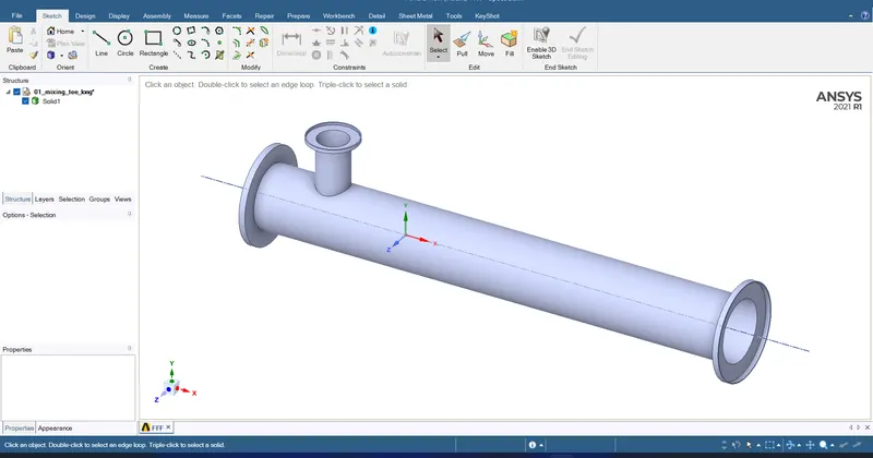
Above figure shows the long mixing tee opened in spaceclaim.

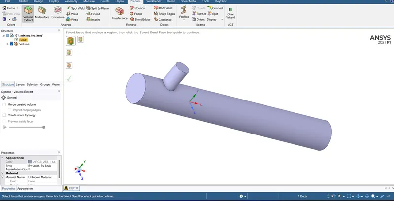
Volume extracted from the model.

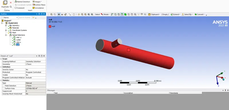
Given name for boundaries

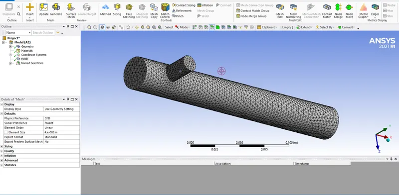
Meshing done with 4mm mesh.

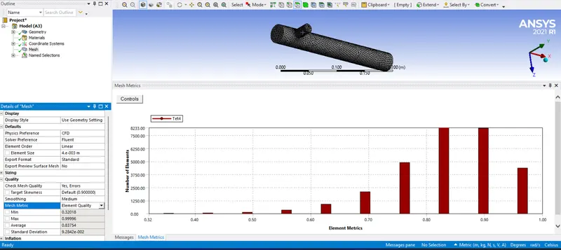
Checking the quality of elements.

Opening the setup window

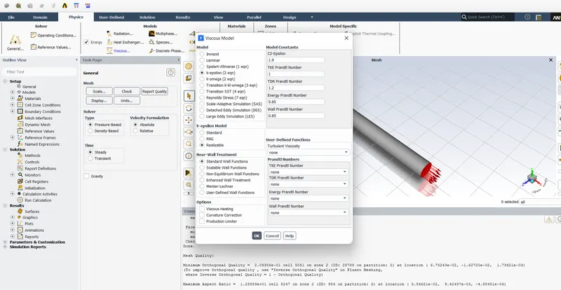
Giving turbulence model

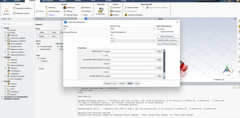
Adding material

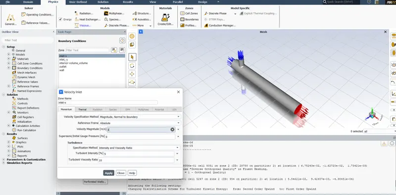
Giving hot inlet velocity as 3m/s

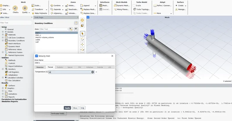
Giving hot inlet temperature as 36 deg.celcius.

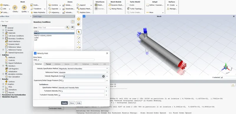
Giving cold inlet velocity as 6m/s

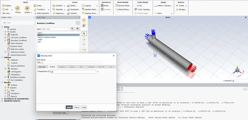
Giving cold inlet temperature as 19 deg.cel.

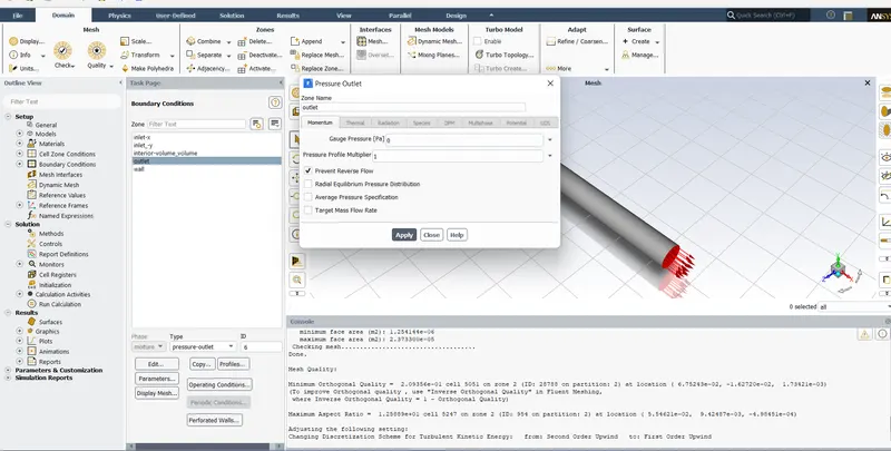
Giving outlet pressure as 0 gauge pressure.

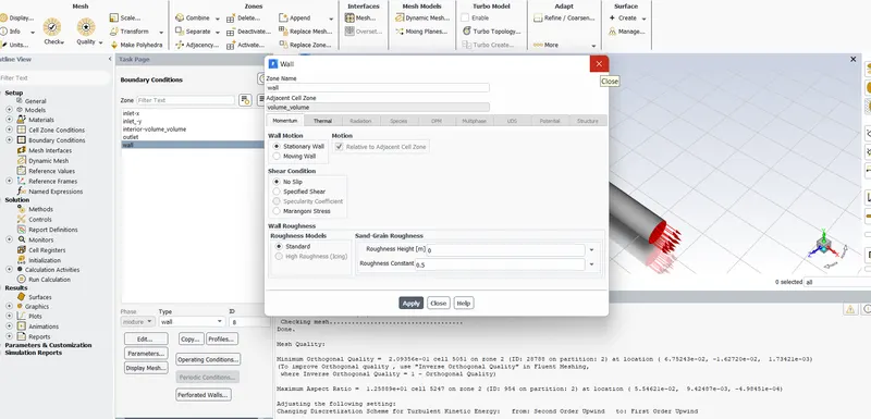
Giving no-slip condition at the wall

Taking area-weighted average of temperature at the outlet

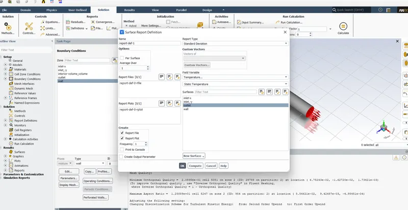
Taking standard deviation of temperature at the outlet.

RESULTS AND DISCUSSIONS:

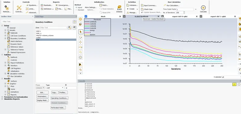
Showing Residuals

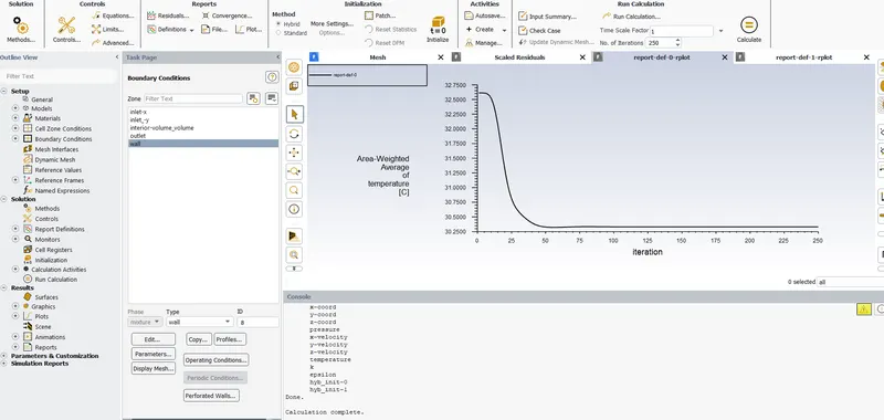
Showing Area-Weighted Average of Temperature at outlet

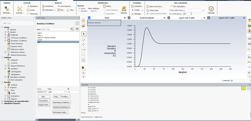
Showing Standard Deviation of Temperature at Outlet

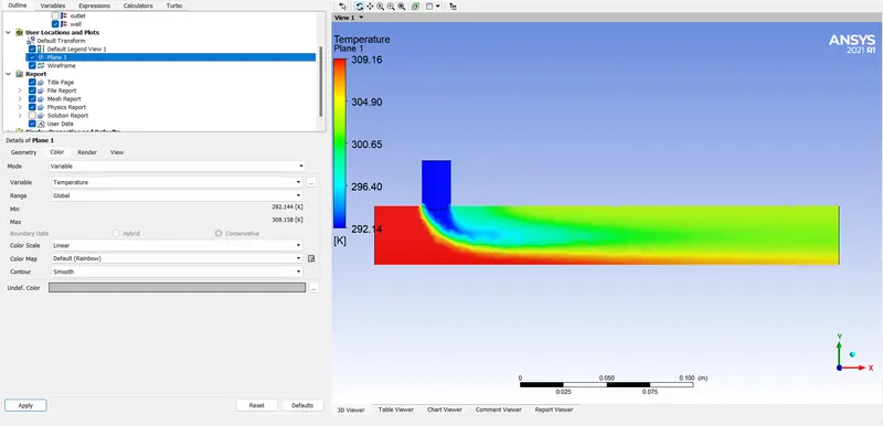
Above figure shows the contour of temperature distribution along the tee.

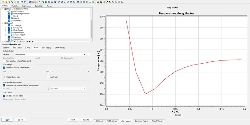
Above figure shows the plot of temperature distribution along the tee.

From the above two figures we can understand that the maximum temperature is around 309.16 K and it is at the left inlet of pipe and minimum temperature is around 292K and which is at the cold inlet.As the result of mixing two flows at the outlet we are getting a temperature around 303K.

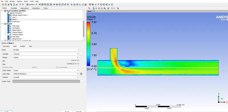
Above figure shows the contour of velocity distribution along the tee.

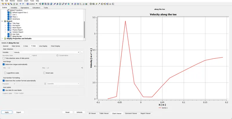
Above figure shows the plot of velocity distribution along the tee.

From the above two figures we can understand that maximum velocity is around 6m/s and which is at cold inlet and minumum velocity is around zero and which near to the wall du to no-slip conditions.At the centre of outlet we are getting a velocity around 3.84m/s

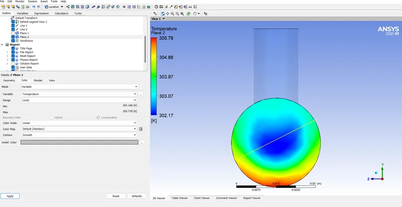
Above figure shows the contour of temperature distribution across the tee.

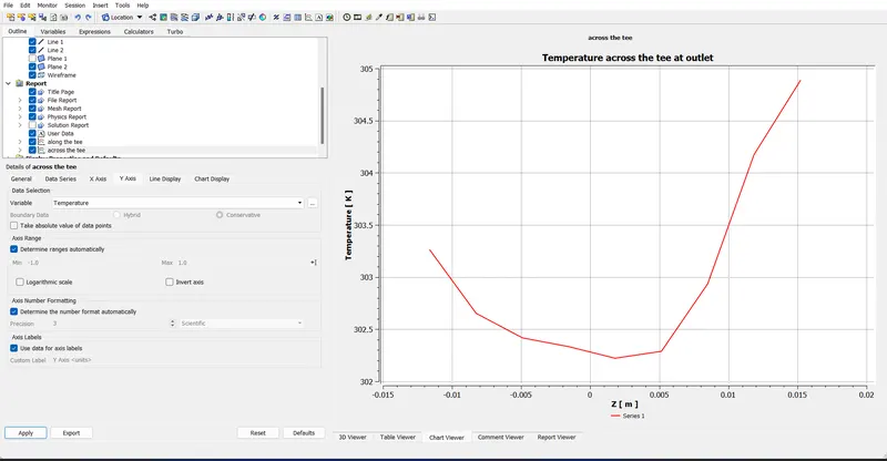
Above figure shows the plot of temperature distribution across the tee.

From the above two figures we can understand that maximum temperature is around 305.50K and which is at bottom part of outlet and minumum temperature is around 302K and which is at the centre of outlet.

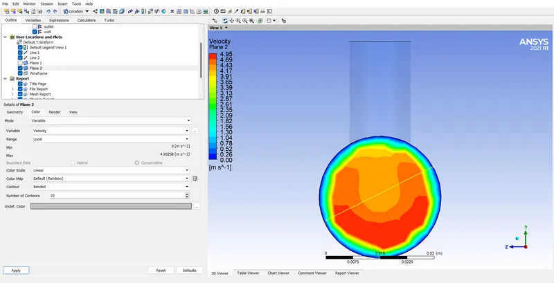
Above figure shows the contour of velocity distribution across the tee.

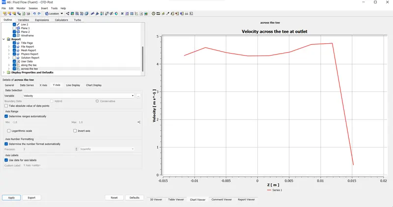
Above figure shows the plot of velocity distribution across the tee.

From the above two figures we can understand that maximum velocity is around5m/s and minumum velocity is around zero and which near to the wall du to no-slip conditions.At the centre of outlet we are getting a velocity around 4m/s

Case 2(b)

• Long mixing tee with a hot inlet velocity of 3m/s.
• Momentum ratio of 4

• RESULTS AND DISCUSSIONS:

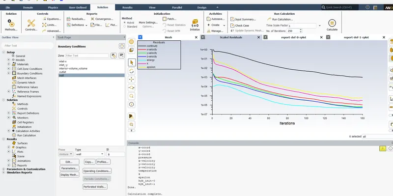
Showing residulas.

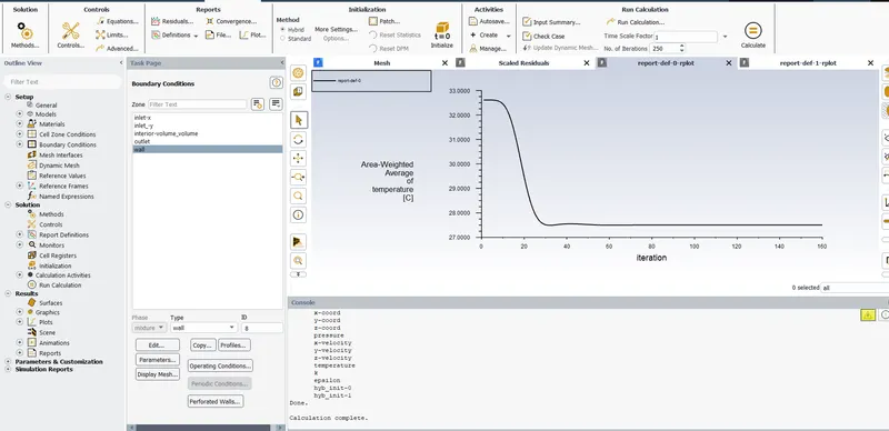
Showing Area -Weighted Average of Temperature at Outlet.(Mean temperature=27.5 deg.cel)

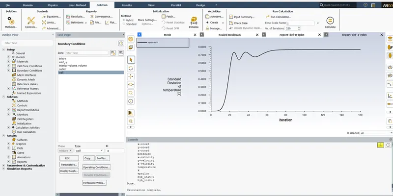
Showing standard deviation of Temperature at Outlet.(Standard Deviation reduces to 0.7)

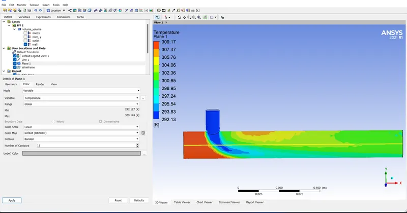
Above figure shows contour of temeprature distribution along the tee.

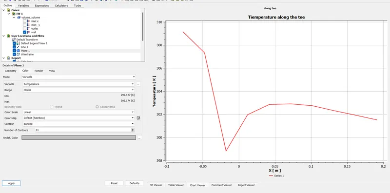
Above figure shows plot of temeprature distribution along the tee.

From the above two figures we can understand that maximum temperature is around 309.17K and minumum temperature is around 292.13K .

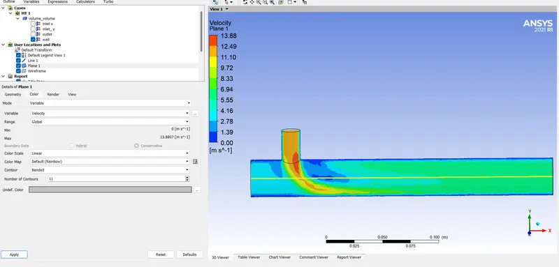
Above figure shows contour of velocity distribution along the tee.

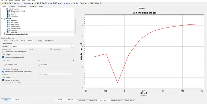
Above figure shows plot of velocity distribution along the tee.

From the above two figures we can understand that maximum velocity is around 12m/s and minumum velocity is around zero at walls due to no-slip conditions.

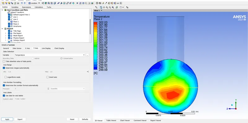
Above figure shows contour of temeprature distribution across the tee.

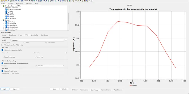
Above figure shows plot of temeprature distribution across the tee.

From the above two figures we can understand that maximum temperature is around 301.7K and minumum temperature is around 299.59K near walls.

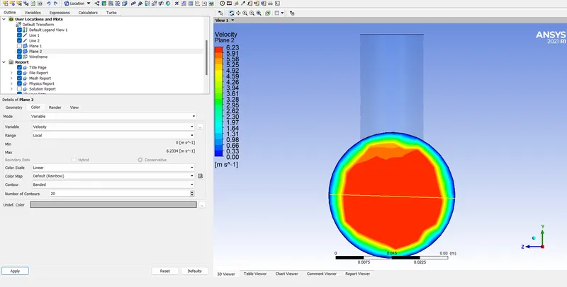
Above figure shows contour of velocity distribution across the te at the outlet.

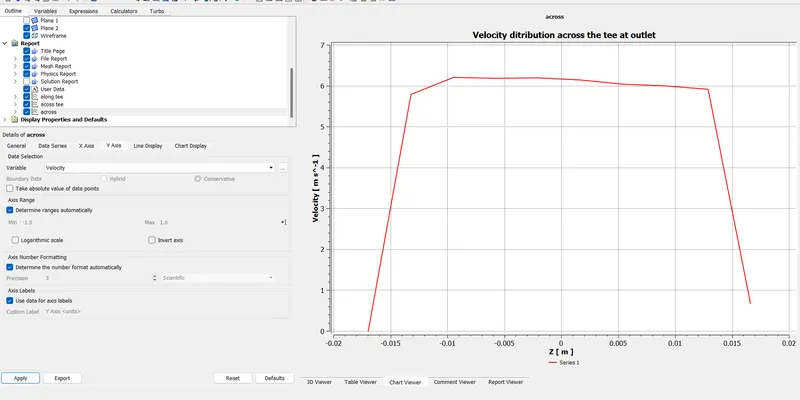
Above figure shows plot of velocity distribution across the te at the outlet.

From the above two figures we can understand that maximum velocity is around 6m/s and minumum velocity is around zero near walls due to no-slip conditions.

COMPARISON :

Cases	Cell Count	Average outlet temperature	Number of iterations for convergence
CASE 1 (a)	39,817	303.25 K	250
CASE 1(b)	39,817	300.5K	160
CASE 1(c)	39,817	301K	180
CASE 2(a)	29,061	303.25K	250

MESH INDEPENDANCE STUDY:

For doing mesh independance study, we are taking CASE 2(b) and for the mesh independance study the parameter taken as is Standard Deviation.

Element Size	Total No of Elements	Standard Deviation
4mm	29,061	0.76525507
2mm	140025	0.81428888
10mm	15368	0.7533932

From this mesh independance study we can understand that standard deviation is varying with number of elements. Standard deviation is getting closer to one when number of elements increasing.

Conclusion:

1. The simulation was run successfully for all cases.

2. For the Case 1(b) case with increased velocity of chilled air the mixing was better and lower temperature was obtained at outlet.

3. The long pipe configuration was not helpful for lower temperature at outlet.

4. There is no much difference in results when we used K-Omega model instead of K-Epsilon model.

5. From mesh independance study we can understand that standard deviation is varying with number of elements. Standard deviation is getting closer to one when number of elements increasing.