Week 1- Mixing Tee

Challenge 1

Aim: - set up steady-state simulations of Mixing tee to compare the mixing effectiveness when hot inlet temperature is 36⁰C & the Cold inlet is at 19⁰C. for Momentum ratio 2 and 4 when hot inlet velocity is 3 m/s

Introduction: - Mixing t is used to mix to fluid we are simulating mixing of air hot air is entering from one end and cold air is entering from another inlet our objective is to find out the outlet temp for different Momentum ratio and length of tee.

Different type of case

1. Case 1
   • Short mixing tee with a hot inlet velocity of 3m/s.
   • Momentum ratio of 2, 4.
2. Case 2
   • Long mixing tee with a hot inlet velocity of 3m/s.
   • Momentum ratio of 2, 4.

Use the k-epsilon and k-omega SST model

Practical application: - practical application of Mixing Tee is used in ac and other fluid mixing application

Procedure: -

• Open ANSYS workbench drag Fluid flow (Fluent) from tool box
• Open geometry using space claim application which shows when right clicked on geometry
• Once spaceclaim application is open import Mixing Tee model which is saved in system first select which type of file is in our system and go to that location and import that file
• Extract only inner volume because our area of interest only on area which is in contact which fluid to do so go to prepare section select volume extract command and extract using edge then select the edge and unselect solid from tree section and supressh that to physics close the space claim
• Click on mesh wait till the application open once open right clich on mesh and click on generate mesh wait till mesh generation
• Once the mesh is generated name face with inlet-, inlet -y, wall and outlet close mesh file
• Click on setup wait till fluent application open
• One the file is open check for mesh from Domain section, in physics section select solver, Type pressure based, velocity formulation absolute and time steady
• In model select energy and in viscous model select k -epsilon model with realization near wall function as standard wall function then click ok
• In materials select air as working fluid
• In zones select boundary conditions for inlets velocity is is given by user and temp also given by used
• In outlet pressure is selected
• Move to solution section in that report select definition for report and write for outlet temp plot and standard deviation plot for outlet temp
• Once done with above steps initialize the solution the calculate the solution for no of iteration the user is interested
• look at the plots of standard deviation and outlet temp
• once calculation done close the application
• click on result once the application is opened select only wall volume and increase the volume transparency
• insert a plane inside the volume wall at the center of the wall and select colour in variable select temp and the temp variation across the pane can be seen
• same process is done for all the cases

Case 2

Long Mixing Tee

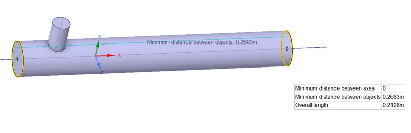
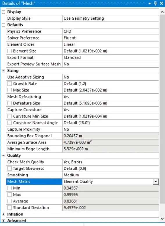
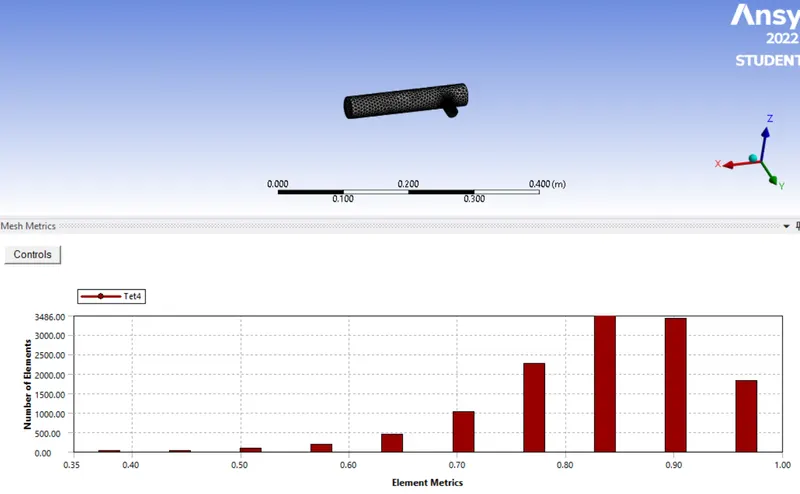
fig 1 mesh Paramers

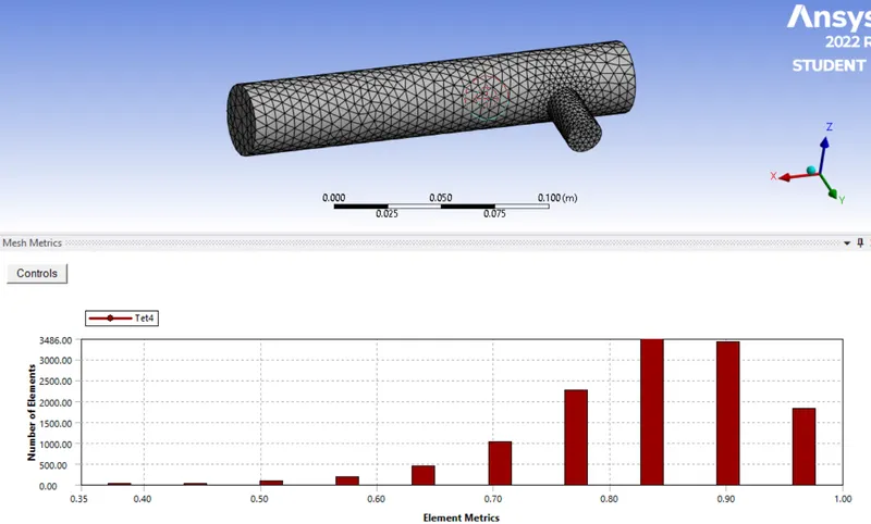
fig 2 mesh quality

k-epsilon model for Momentum ratio 2:- convergerd atMomentum ratio168 th iteration

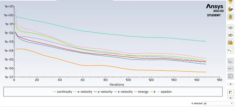
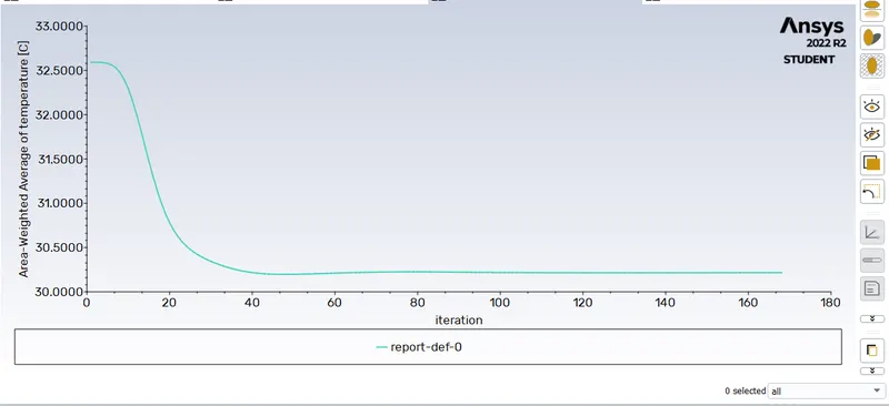
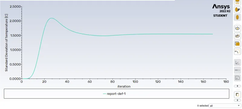
fig 3 iteration vs velocity,countinuety,outlet temp and standard deviation plot

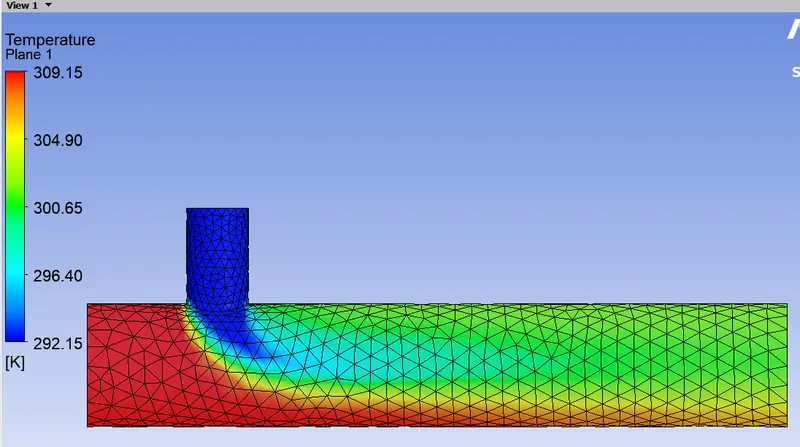
fig 4 result plot of k epsilon viscus model

k-oega model for Momentum ratio 2:- convergerd at 256 th iteration

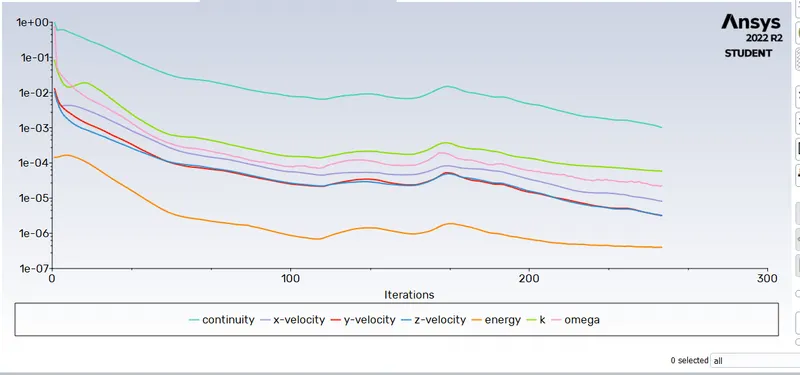
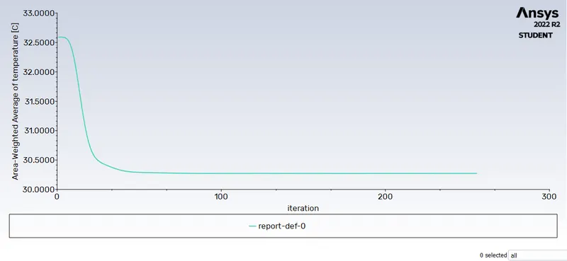
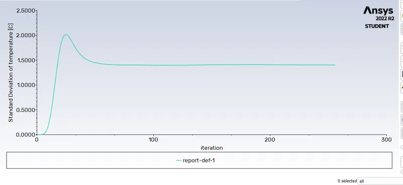
fig 5 iteration vs velocity,countinuety,outlet temp and standard deviation plot

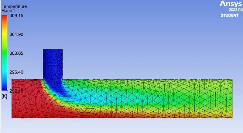
fig 4 result plot of k Omega viscus model

k-epsilon model for Momentum ratio 4:- convergerd at 154 th iteration

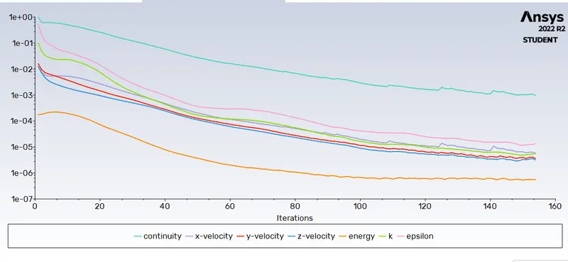
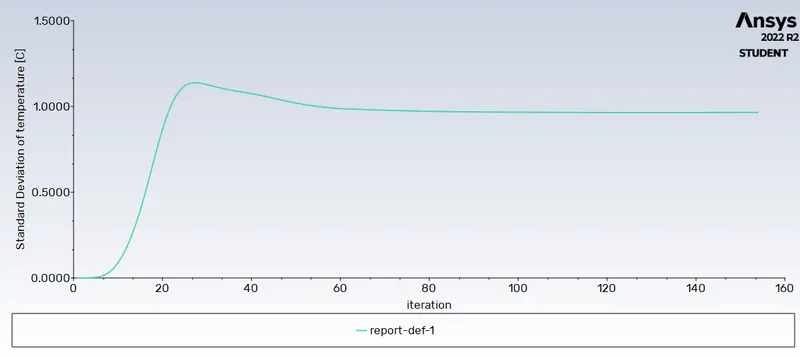
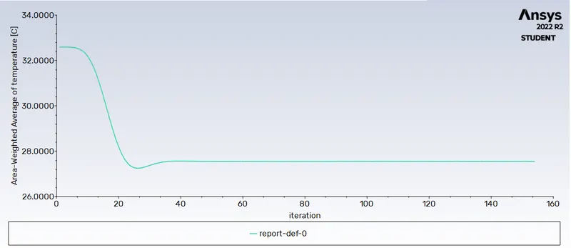
fig 6 iteration vs velocity,countinuety,outlet temp and standard deviation plot

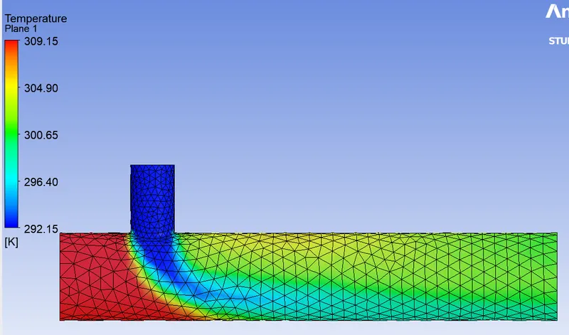
fig 7 result plot of k epsilon viscus model

k-omega model for Momentum ratio 4:- convergerd at 138 th iteration

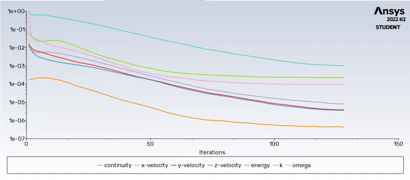
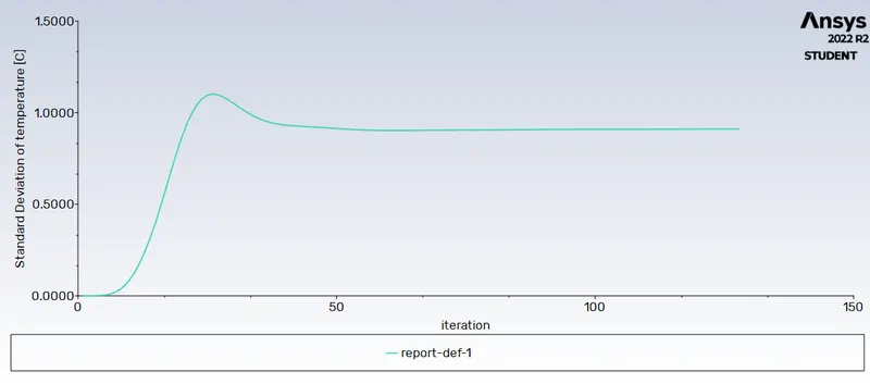
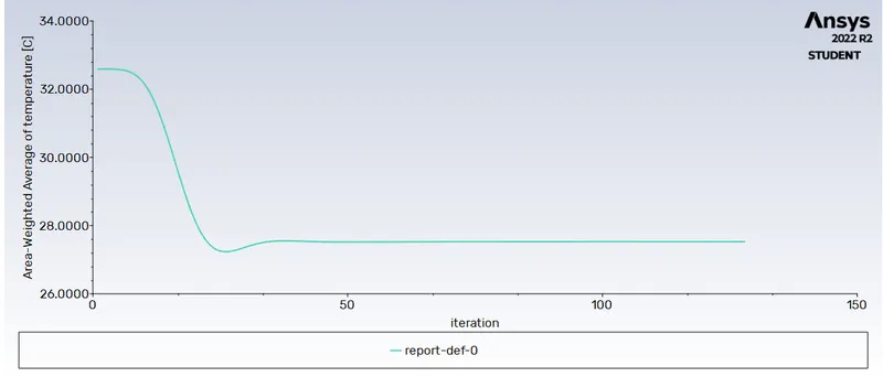
fig 8 iteration vs velocity,countinuety,outlet temp and standard deviation plot

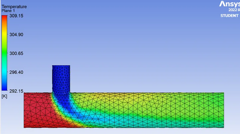
fig 4 result plot of k omega viscus model

case-1: Short Mixing Tee

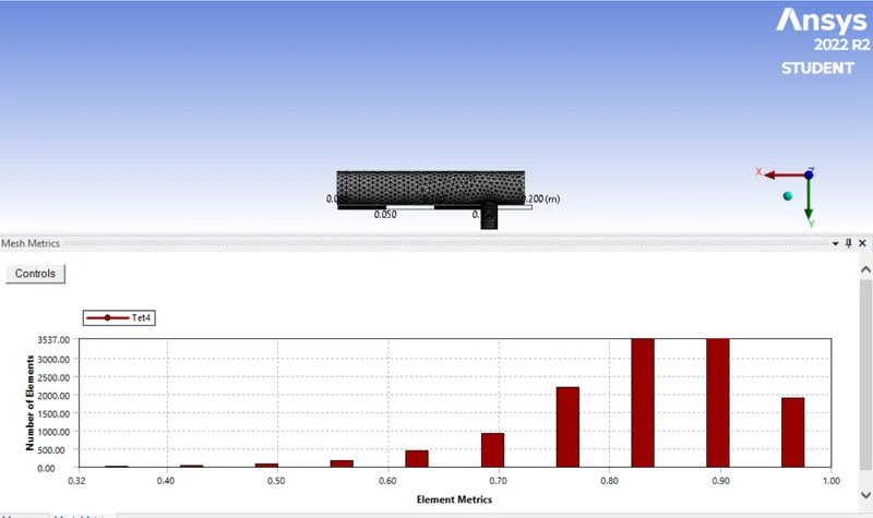
fig 9 mesh quality

k-epsilon model for Momentum ratio 2:- convergerd at150 th iteration

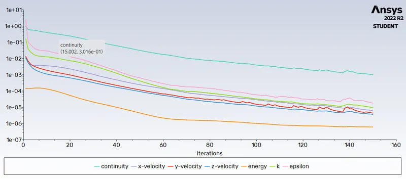
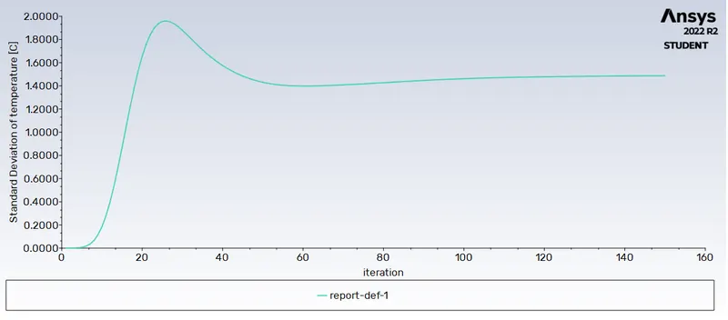
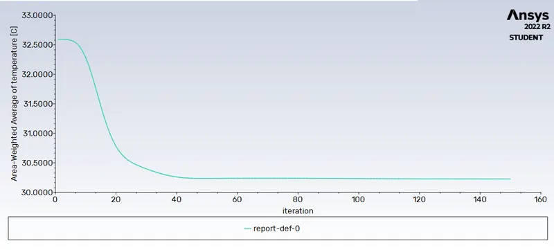
fig 10 iteration vs velocity,countinuety,outlet temp and standard deviation plot

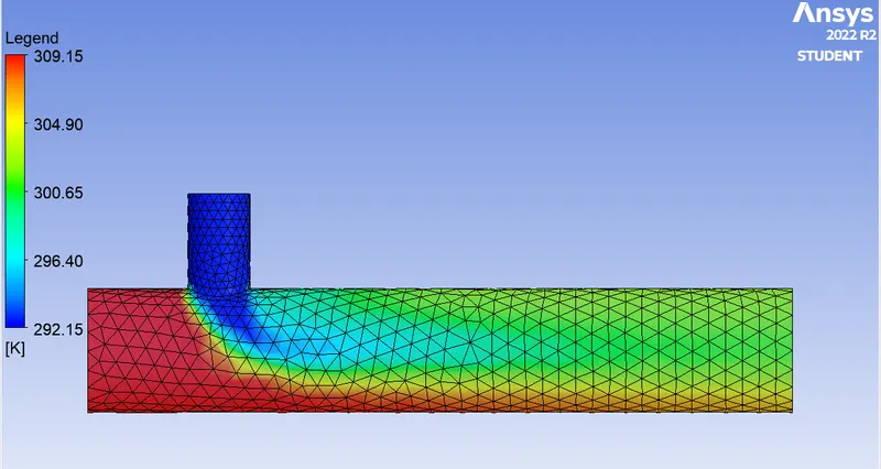
fig 11 result plot of k epsilon viscus model

k-omega model for Momentum ratio 2:- convergerd at 287 th iteration

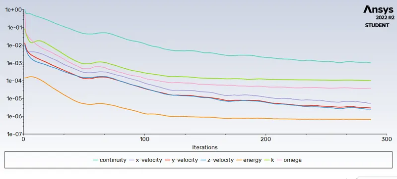
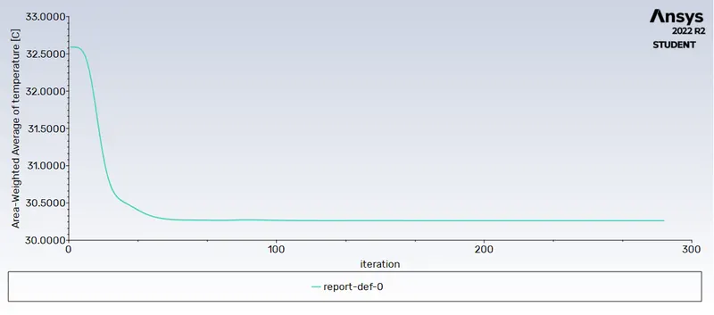
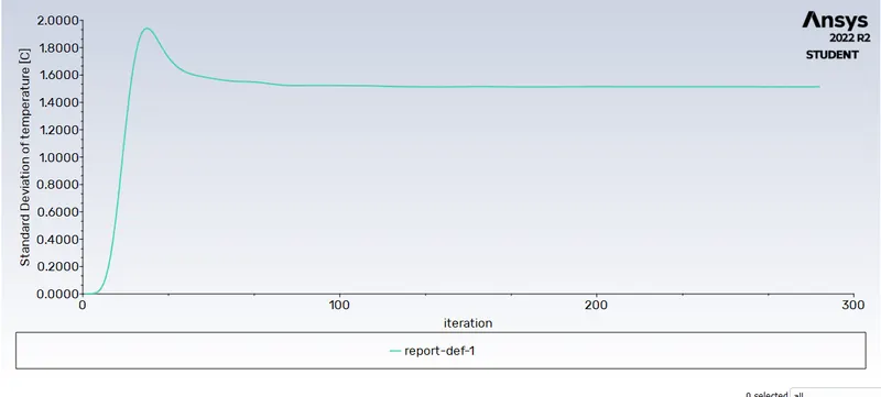
fig 12 iteration vs velocity,countinuety,outlet temp and standard deviation plot

k-epsilon model for Momentum ratio 4:- convergerd at 245 th iteration

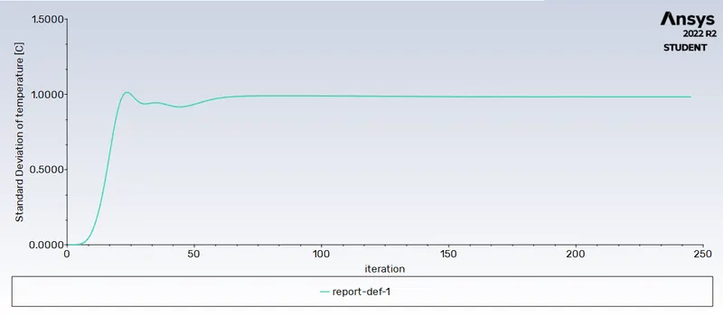
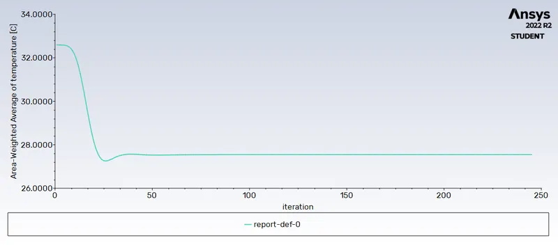
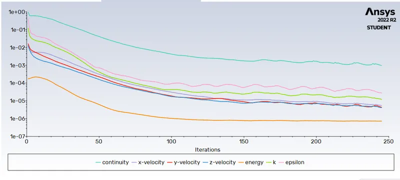
fig 13 iteration vs velocity,countinuety,outlet temp and standard deviation plot

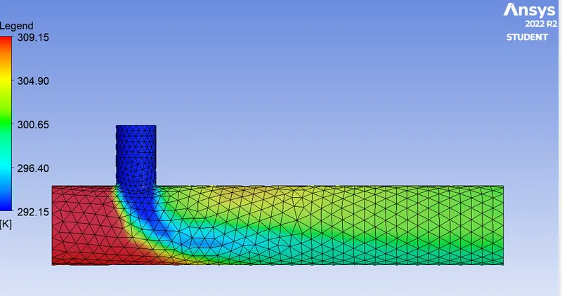
fig 14 result plot of k epsilon viscus model

k-epsilon model for Momentum ratio 4:- not convergerd

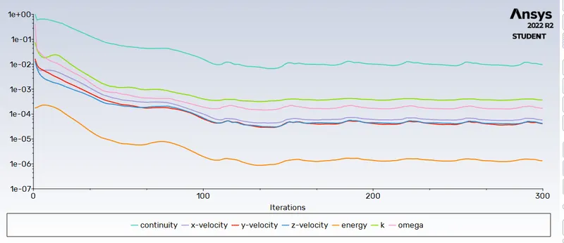
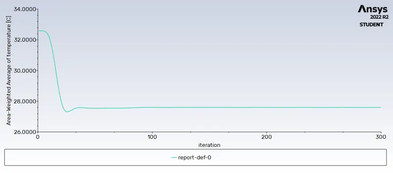
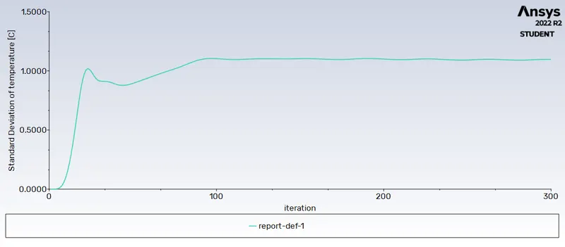
fig 15 iteration vs velocity,countinuety,outlet temp and standard deviation plot

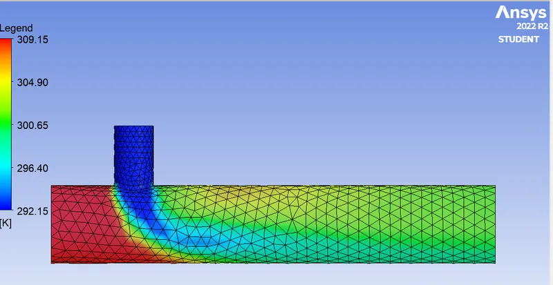
fig 16 result plot of k epsilon viscus model

conclusion: -

from above 2 case study it can be seen that when the length of the Tee section increased there is not much effect on the outlet temp but when the Momentum ratio changed there is significant change in the outlet temp

where as with viscous model concern there is only change in conversion time and iteration took to converge but the result remain same for temp variation