Week 1- Mixing Tee

AIM:

• To setup a steady state simulation of a mixing Tee and study the effectiveness of the mixing due to varying lengths.
• To apply the k-epsilon and k-omega models for simulation and determine the best suited method to be adopted.

K-`omega` MODEL

The k-omega turbulence model is one of the most commonly used models to capture the effect of turbulent flow conditions. It belongs to the Reynolds-averaged Navier-Stokes (RANS) family of turbulence models where all the effects of turbulence are modeled.

It is a two-equation model. That means in addition to the conservation equations, it solves two transport equations (PDEs), which account for the history effects like convection and diffusion of turbulent energy. The two transported variables are turbulent kinetic energy (k), which determines the energy in turbulence, and specific turbulent dissipation rate (`omega`), which determines the rate of dissipation per unit turbulent kinetic energy. `omega` is also referred to as the scale of turbulence.

The standard k-`omega` model is a low `Re` model, ie., it can be used for flows with low Reynolds number where the boundary layer is relatively thick and the viscous sublayer can be resolved.

K-`epsilon` MODEL

The k-epsilon model for turbulence is the most common to simulate the mean flow characteristics for turbulent flow conditions. It belongs to the Reynolds-averaged Navier Stokes (RANS) family of turbulence models where all the effects of turbulence are modeled.

It is a two-equation model. That means that in addition to the conservation equations, it solves two transport equations (PDEs), which account for the history effects like convection and diffusion of turbulent energy. The two transported variables are turbulent kinetic energy (K), which determines the energy in turbulence, and turbulent dissipation rate (`epsilon`), which determines the rate of dissipation of turbulent kinetic energy.

The K-`epsilon` model is shown to be reliable for free-shear flows, such as the ones with relatively small pressure gradients, but might not be the best model for problems involving adverse pressure gradients, large separations, and complex flows with strong curvatures.

Analysis of the Short mixing tee using the above two methods:

Upon analysing the results, it was found that the K-`omega` method had provided stable results compared to the K-`epsilon` method. This is because, the latter is a high Reynold's number solver. However, when we consider the temperature standard deviation as a parameter, either methods provide us with similar results. Thus, in this case, either method can be used to estimate the results.

PROCEDURE TO SETUP THE CASE:

• The Ansys workbench application is opened and the fluent module is selected.
• The profile is initially loaded into Space Claim. In order to load the profile, it must be in any of the acceptable extension by space claim. In this case it was a solidworks file.
• The volume of the model is extracted using the volume extract function in the prepare section of space claim.
• We select the edges of the model inorder to form the required volume extract.
• Further more we make sure that the actual model is suppressed for physics to ensure that the analysis is done on the volume extract.
• The space claim file is then closed.
• The meshing file is opened and the requsite dimension of the mesh is inputed and generated. Then we create names to the edges namely inlet-x, inlet-y etc as required. This simplifies applying boundary conditions in the setup a Ansys automaticaly assigns type dependant on the names provided.
• The geometry is then sectioned by using the plane option to ensure that the simulation is run on the sectioned portion.
• Setup is done as per requirement.
• The required plots are selected and the other requsite steps are performed.
• After running the simulation, the results are obtained and studied.
• Post processing is opened and the the solution is studied. We study the parameters by creating a plane.
• In this module we study the variation of various factors in this case temperature and velocity.

SHORT MIXING TEE:

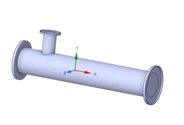
Short Tee Profile

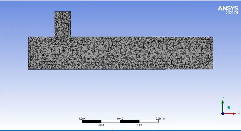
Mesh dimension 2e-3

CASE 1: Short Tee

Case 1-a: grid size: 2e-3 and momentum ratio 2:

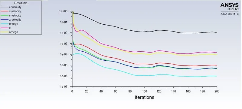
Residual plot:

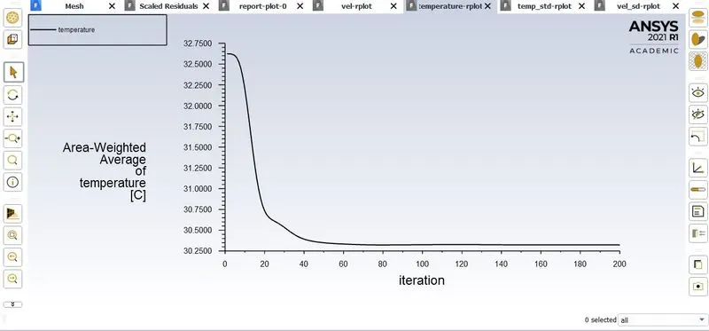
Temperature Plot:

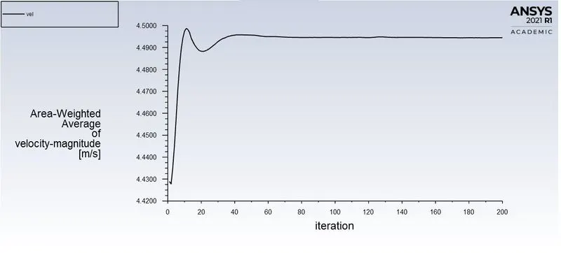
Velocity:

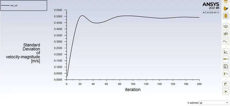
Standard Deviation:

PROFILES:

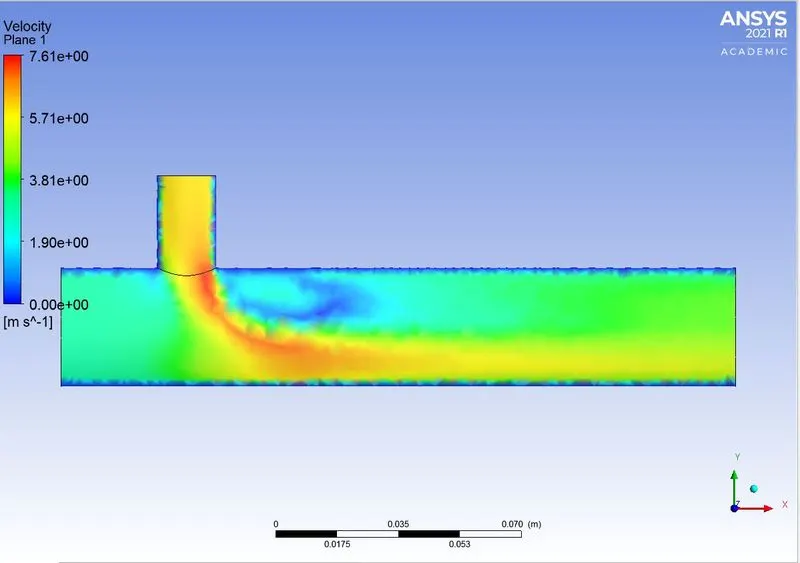
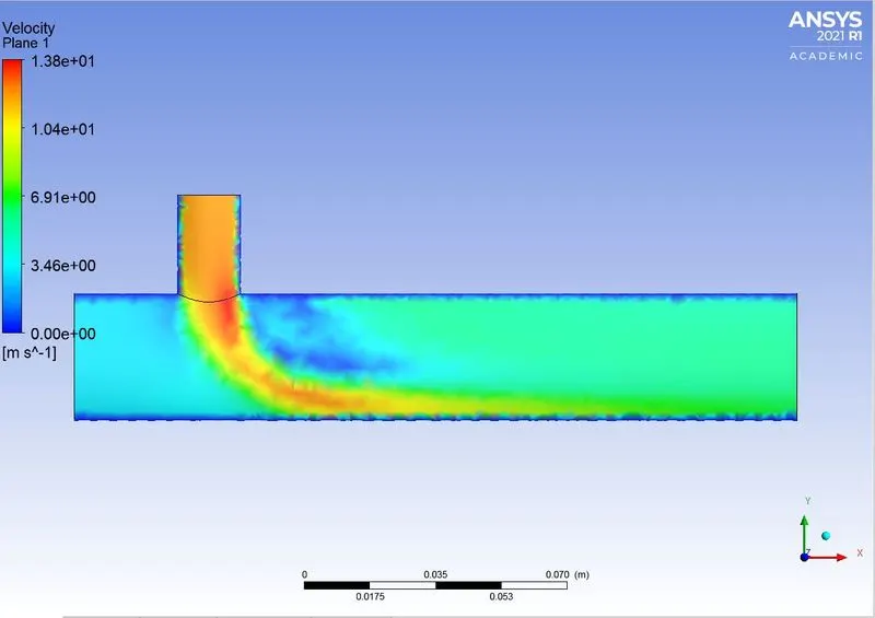
Velocity:

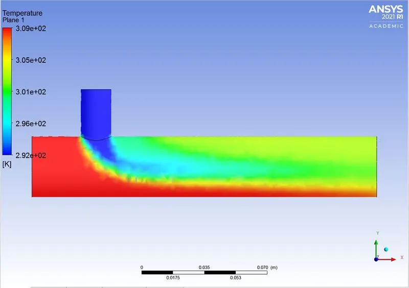
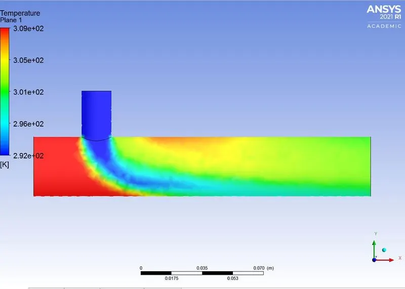
Temperature:

Case 1-b: Short mixining tee with momentum ratio 4:

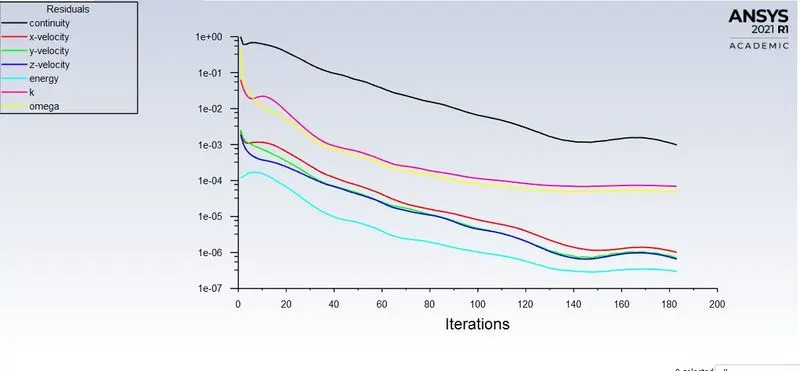
Residuals plot:

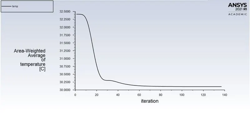
Temperature plot:

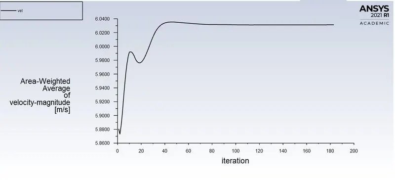
Velocity:

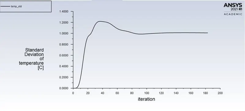
Standard Deviation:

PROFILES:

Velocity:

Temperature:

Case 2: LONG TEE:

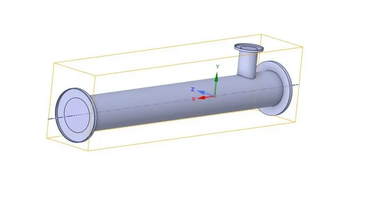
Long Tee Profile

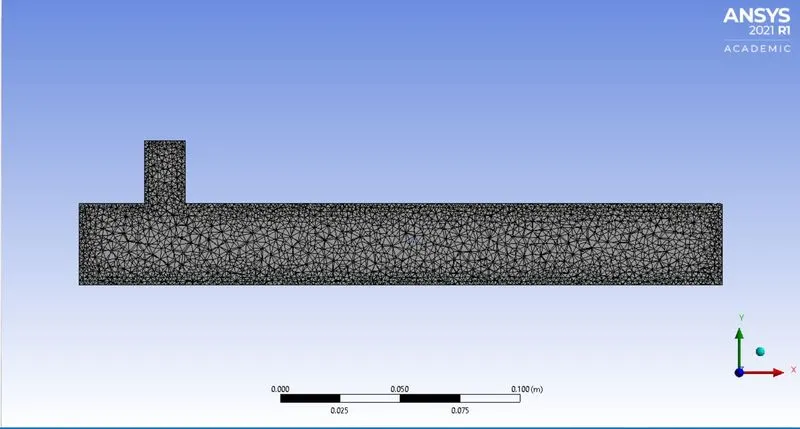
Mesh Size 2E-3

Case 2-a: Long tee with momentum ratio 2:

Residual plot:

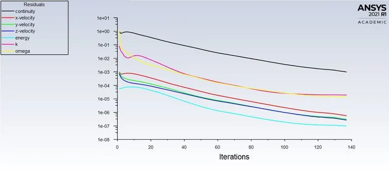
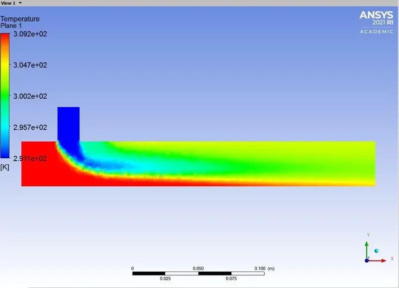
Temperature plot:

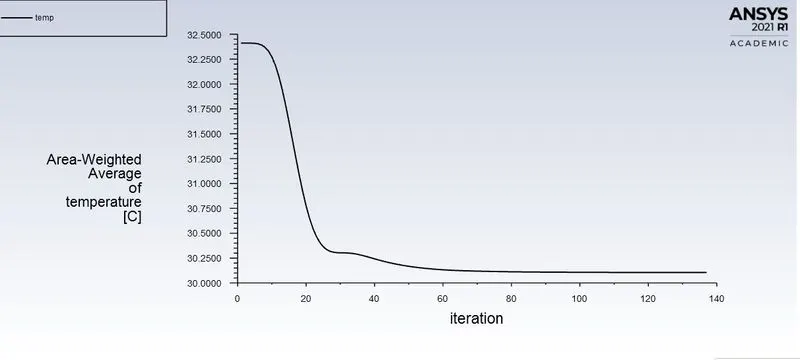
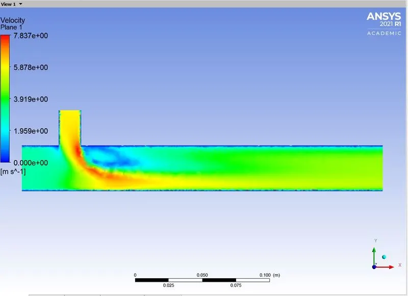
Velocity Plot:

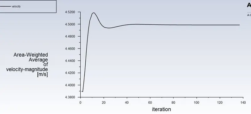
Standard Deviation:

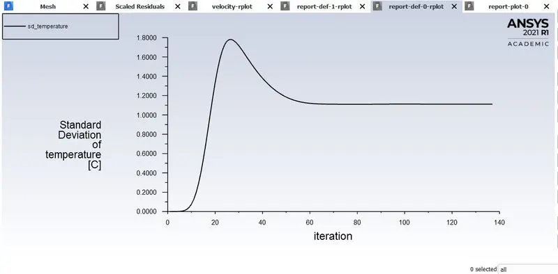
PROFILES:

Velocity:

Temperature:

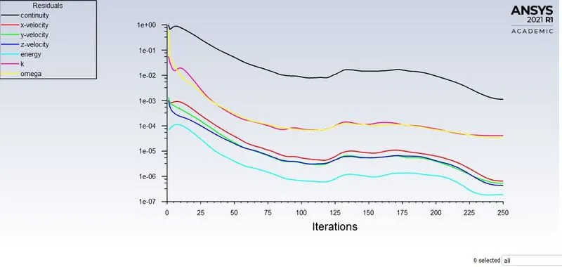
Case 2-a: Long tee with momentum ratio 4:

Residual plot:

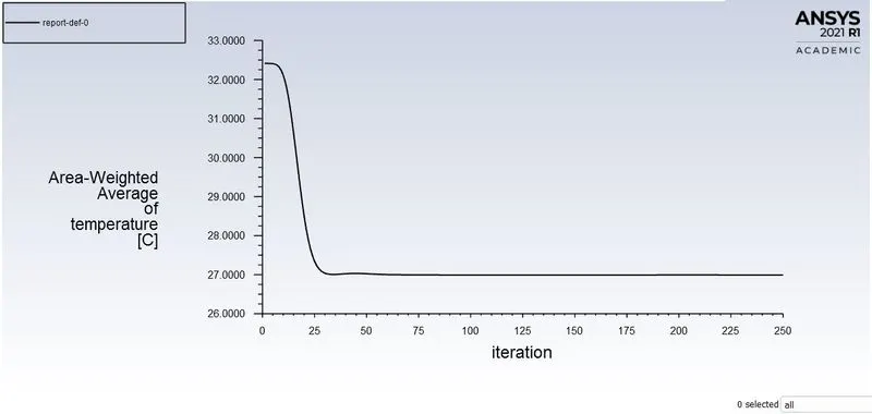
Temperature plot:

Velocity Plot:

Standard Deviation:

PROFILES:

Velocity:

Temperature:

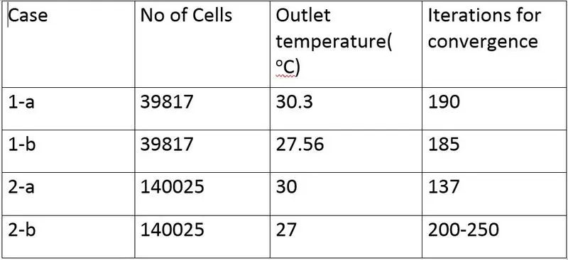
COMPARISION OF THE CASES:

INFERENCE:

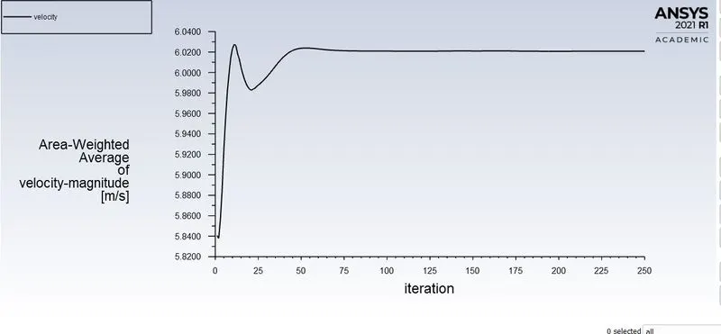
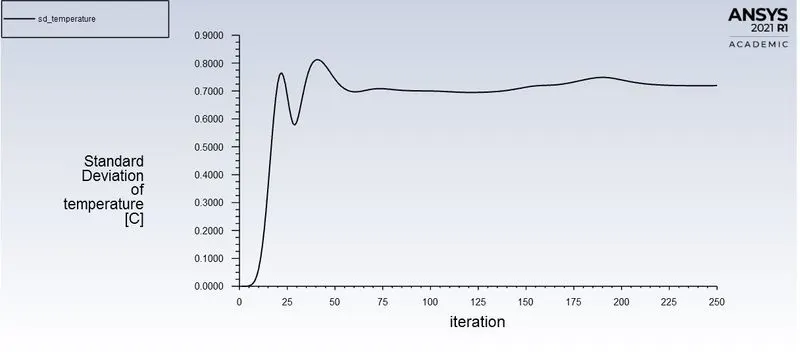
• From the above results, we can conclude that there seems to be better mixing in the for case 1-a and case 2-b by observing the standard deviation plots.
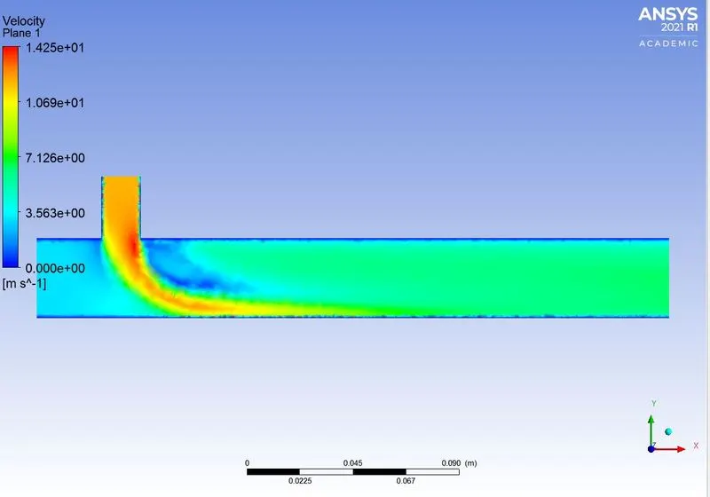
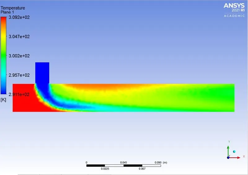
• However, we can observe that when the velocity of the cold air is increased, there is a significant decrease in temperature is noted. This happens due to effective mixing of the air at room temperature and the cool air.
• There is neglegible difference in outlet temperature in the cases of 1-b and 2-b. So the use of Short tee with increased inlet velocity is best for the applications.