Week 1- Mixing Tee

Aim: Flow through Tee_joint

Medium of Flow:Air, through pipe flow (aluminium)

Properties of air:

• Density
• Specific heat
• Thermal conductivity
• viscosity
• Molecular weight
• State Entropy
• Temperature
• Charcateristic length
• Pressure
• Specific Volume
• Momentum
• velocity
• mass

Properties of Aluminium:

• Density
• Specific heat
• Thermal Conductivity
• mass

Boundary's of Geometry:

• Two inlets ports
• One outlet ports
• Walls

Boundary conditions:

Given are:Dirichilet : Specifying values of Condition

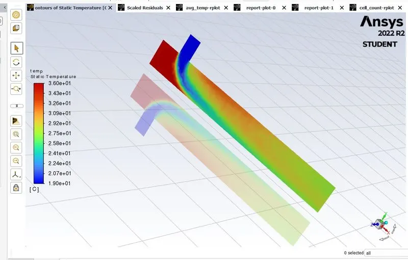
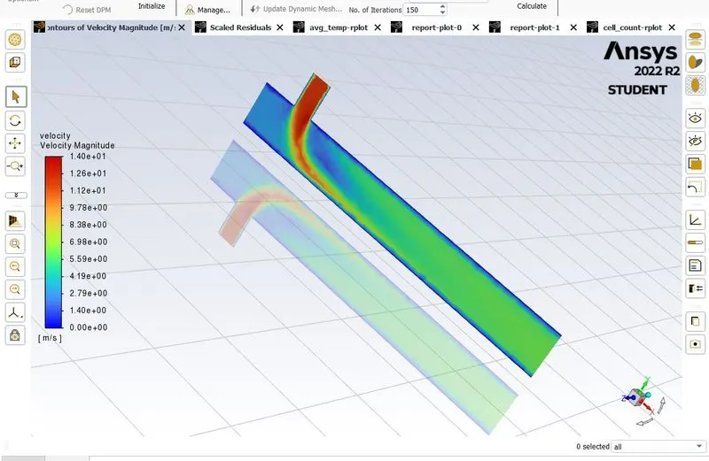
• Velocities and Temp at Inlet ports
• Zero pressure at oulet port

To find: Temperature at outlet

My Observation:

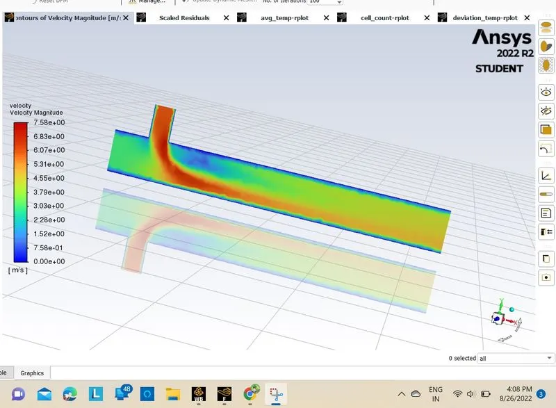
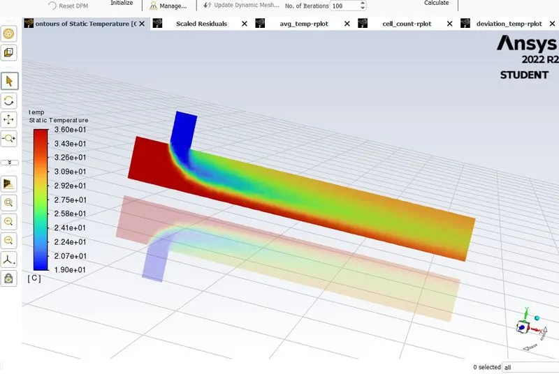
• The working fluid material is air flowing through an aluminiun pipe with some different Intial velocities & temp with chilled air & Normal air,after entering into the pipe the flow at initially makes Laminar(movement of layers) ,if velocity of flow increases it may turn to Turbulent flow (movement of Eddies).

1. Case 1
   • Short mixing tee with a hot inlet velocity of 3m/s.
   • Momentum ratio of 2

Calculation complete.

Area-Weighted Average [C]

-------------------------------- -------------------

outlet_x 30.222687

Standard Deviation [C]

-------------------------------- -------------------

outlet_x 1.3669415

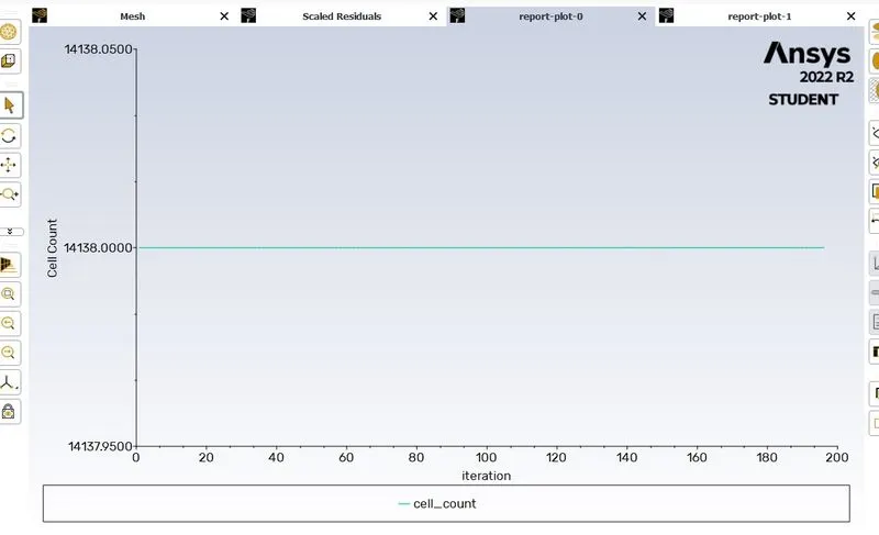
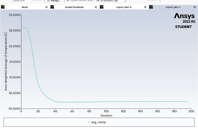
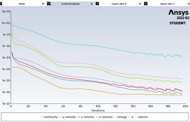
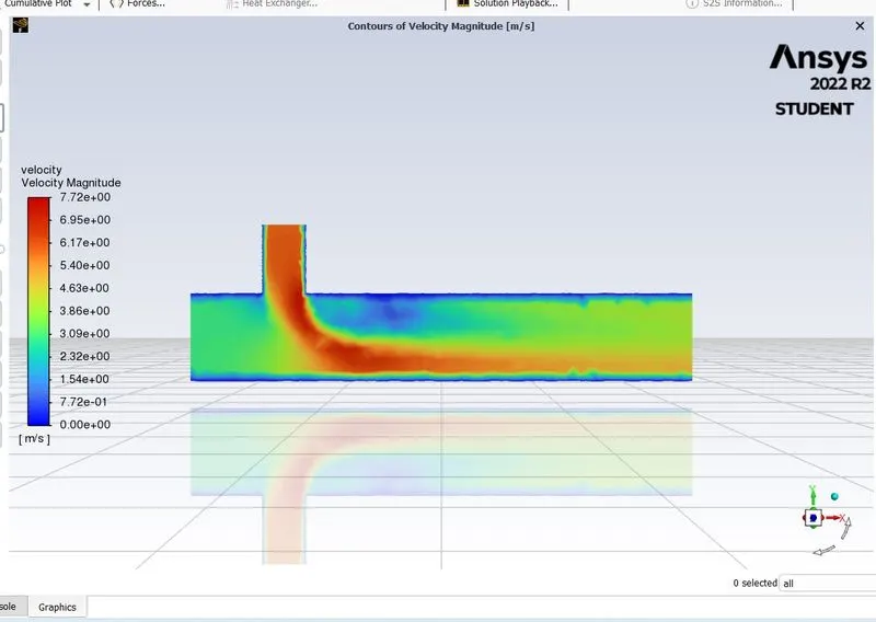
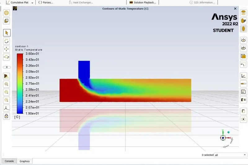Case 1

• 
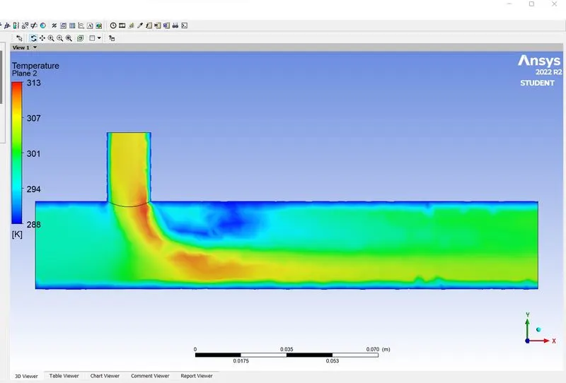
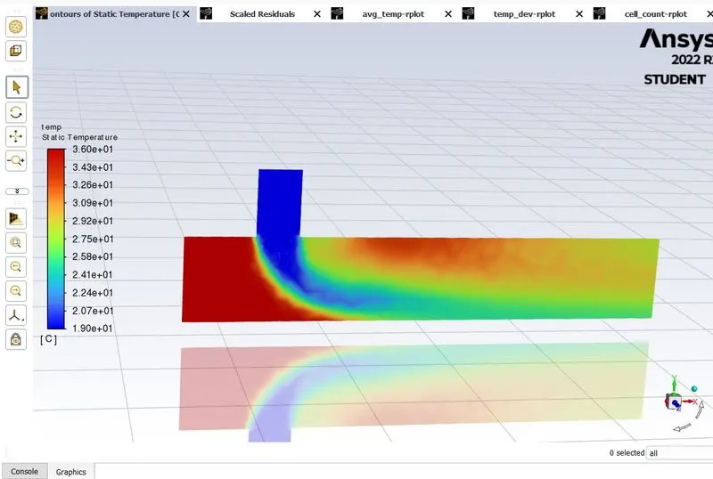
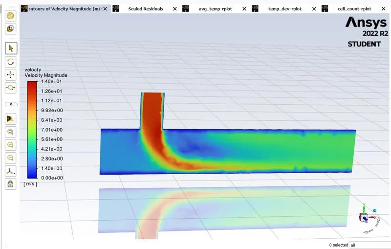
• case2
• Short mixing tee with a hot inlet velocity of 3m/s.
• Momentum ratio of 4

Calculation complete.

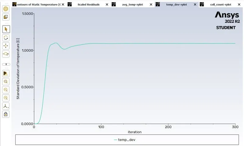
temp_dev

-------------------

Standard Deviation [C]

-------------------------------- -------------------

outlet_x 1.093839

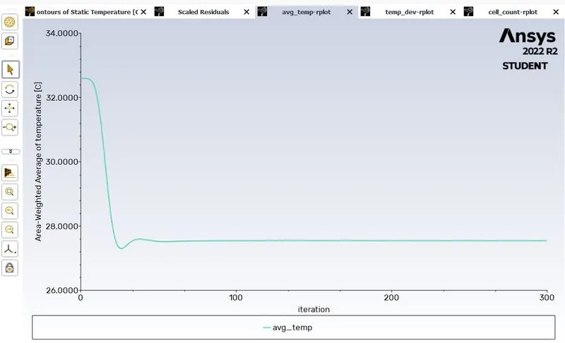
avg_temp

-------------------

Area-Weighted Average [C]

-------------------------------- -------------------

outlet_x 27.543792

Case3:

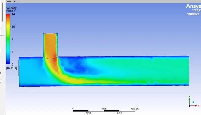
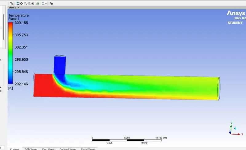
• Long mixing tee with a hot inlet velocity of 3m/s.
• Momentum ratio of 2

Calculation complete.

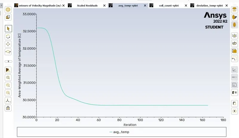
avg_temp

-------------------

Area-Weighted Average [C]

-------------------------------- -------------------

outlet_x 30.342898

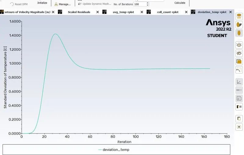
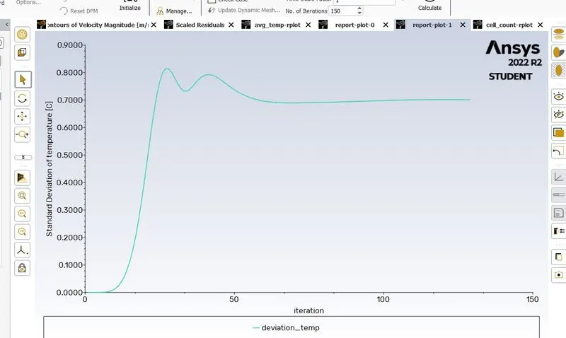
deviation_temp

-------------------

Standard Deviation [C]

-------------------------------- -------------------

outlet_x 0.92529185

Case4:

• Long mixing tee with a hot inlet velocity of 3m/s.
• Momentum ratio of 4

Calculation complete.

deviation_temp

-------------------

Standard Deviation [C]

-------------------------------- -------------------

outlet_x 0.70111544

avg_temp

-------------------

Area-Weighted Average [C]

-------------------------------- -------------------

outlet_x 27.477181

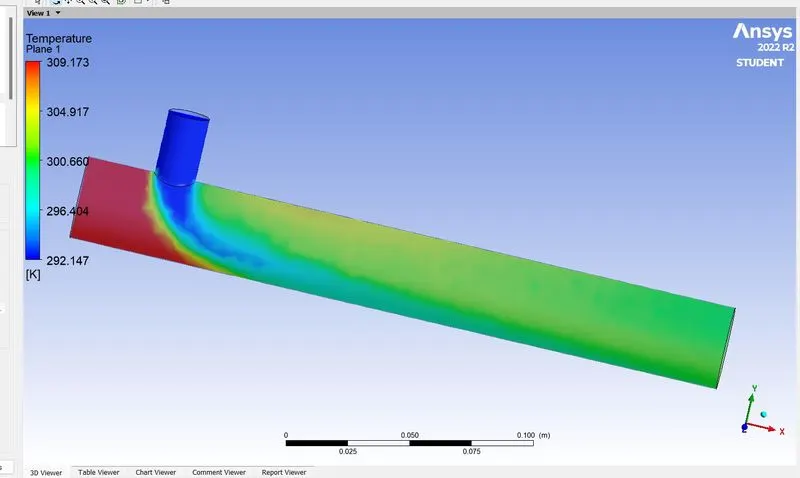
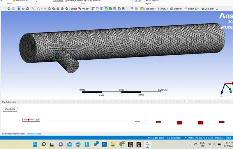
• Most fluids flow problems are non Linear in nature dealing with inheritently Unstable phenomeana such as Turbulence.
• The solution Technique Uses iterative process to successively improve a solution Until Convergence is reached

About Convergence:

Study of CFD Engineer:To study the iterations b/w the equations.

Judgement of CFD analyst:The point at which the analysis Deemed.ie, Converged.

• When your Simulation has no change on all the Convergence criteria after certain Iterations or timesteps,then we conider solution has reached a Steady_state ie., Converged.
• In Mathematics Convergence describes an limiting behevior particularly of an infinite sequence or series towards some limit.
• To declare Convergence is to claim Existence of limit which may itself Unknown,ie., the exact solution to the iterative problem is Unknown,but you want to be sufficiently close to that solution for a particular level of accuracy.So, Convergence therefore does,need to be associated with requirement for a particular level of accuracy.This requirement depends upon the purpose to which the solution will be applied.
• Convergence which called as Bugetary convergence ie., which your solution is Converged,you cant afford any more Computing time.

Convergence of Steady_state CFD analysis: The following 3 Convergence criteria analysis process to be done

They are 1.Residuals.

2.Solution Imbalences.

3.Quantity of interest.

Convergence criteria's:

Continuity eq

x-velocity

y-velocity

z-velocity

Energy eq.

Turbulence eq.

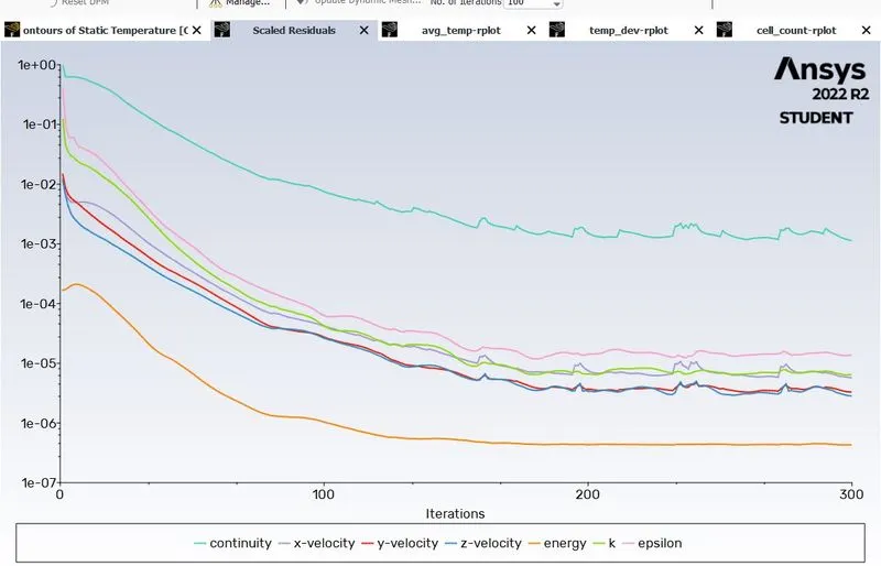
1.Residulas values: The Residual is the most fundamental measures of iterative solution Convergence.

• The Residual Measures the imbalances of Conserved variable's (Mass,Momentum, Pressure,Turbulence) in each controlled Volume,Therefore Every cell in your model will have its own residual value for each of equation's being solved.

• When we are doing CFD Simulations and solving bunch of Governing eq's are Partial differntials/Differntials are going to be form ie., for which Sum Function is equal to zero ,So Functions on Computer will employ as Kind of Approximation and that what is called as Numerical Approximation which, in this case is called Finite volume method.

• We Use FVM approach to discretize partial differntial eq's to solve it , actually the Function will not evluate to Zero, its evaluate something really small to 1e-5 that is called Residuals. ie., for iterative numerical solution the residual will never be exactly zero. however the lower residual value is,the solution is more numerically accurate.

• As no of iterations Continue, what we are seeing here,the functions are calculated very very close to zero.

• Remember your fluid dynamic eq's are solved in each & every cell,the more no of cells ,the more no of equations need to be solve and also the Simulation time increases.

• As we add more cells(fine mesh) the solver is going to take more iterations/timesteps to converge, where is mesh is few no of cells(Coarse mesh) then converge prity fast.

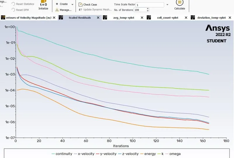
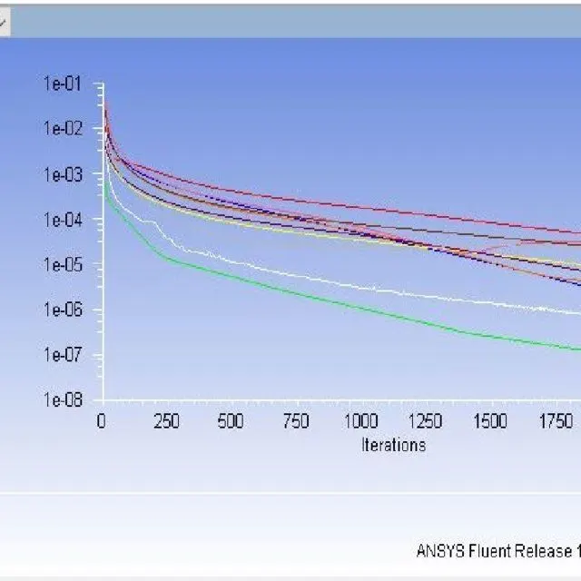
• All residuals get plotted on one graph with y_axis as LOGscale.
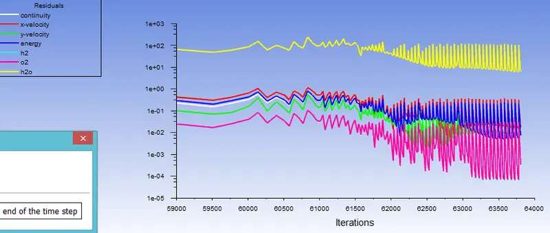
• In analysis plot there will be plot called Residual plot ,the role of this plot is to monitor the change in each and every Convergence criterian for every timestep & plot this values for every iteration or timestep.

• The Key element to identify the Residual is Decreasing lines,Downward slopes,ie.,Residual always to decrease.

• RMS Residual levels of 1E-4 are lossely connected,Residual levels of 1E-5 are well converged,& levels of 1E-6 are tightly converged.

Steady state plot

Unsteady_state plot

2.Solution Imbalances:

• As the word Conservation suggests,the quantities from Conservation eq's (Mass, Momentun,Energy ) should conserve till the last iteration.
• The solution imbalances will never be exactly zero because we are representing the physical system into an algebraic (numerical) form.however the imbalances sufficiently small before considering the solution is converged.
• The solution imbalances gradually decrease as solution progresses.In general small value of residuals leads to small solution imbalance

3.Quantity of Interest:

• In an iterative problems ,the calculation process starts with initial estimations on quantities,like Velocity,pressure,temp etc.,
• In every iterations the Quantities are updated with respect to the previous iteration results.

• In converged steay_state solution, one should expected to see those quantities come to an expected level & dont change any more.
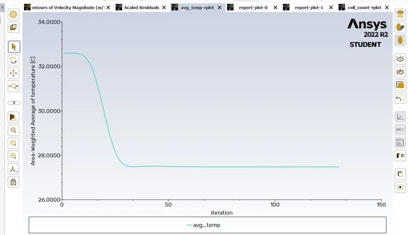
• Monitoring Integrated Quantities like Force, Drag ,avg temp can help the user once his or her analysis has reached this point,there might be instances one quantity may have reached its final point,yet other shows signs of Fluctuations.
• Its better to iterate to the point where values are flatten out in order to consider solution is converged.

We know above fig tells temp after 35 iterations is within just a few percents to its final value,once the monitor point values have" Flattened out"we can safely asssume the sol is converged.

Results of Poor Convergence:

• Diverged sol.
• stuck residuals.
• Increaing imbalances.
• Unstable sol.

Imp points:

Troubleshooting Residuals:

• The Residuals for single equations go bad ,look for trouble spots in the mesh.
• If Residuals are constantly bad, change the order of interpolation.
• If Residuals are oscillating & not showing a Downward trend,try reducing order_relaxation Factor.
• For the density based solver reduce Courant number.

To decrease Numerical Error:

• Using highorder discretization schemes decrease numerical error
• Interpolation errors decrease with decreasing cell size.
• Truncation error is minimized in a uniform Mesh.
• Minimize cell skewness & aspect ratio
• Avoid aspect ratios higher than 5.1
• Maintain Optimal quad/hexa cell angle as 90 degrees,Optimal tria/tetra cell angle as 60 degress.
• Aligning grid with the flow to minimize the Diffussion.

About Turbulence:

• Most Flows occuring in nature are turbulent.
• Many Turbulent flows can be observed easily ,like clouds,occean currents,gulf streams,flow over aircraft wingsetc.,
• Describing Turbulence its refer to Eddymotion which is local Swirling motion, ie., Vorticity.
• The Vorticity field is the curl of velocity field and is twice the rotation rate of fluid particles.
• Turbulent eddies of wide range of sizes appear and give rise to vigorous Mixing (ie,,. sequence of the mixing of Momentum)
• Arc flows
• Most of Dynamics of turbulence is the same in all fluids (liquids and gaseous)
• If Reynolds no larger enough major characteristics of turbulent flows are not controlled.
• Since the equations of motion are non_linear flow characeristics that are associated with its initial and Boundary conditions.

Origin of Turbulence:

• In flows, which are originally laminar,Turbulence arises from instabilities at large Reynold's no
• Turbulent cannot maintain itself but depends on its environment to obtain energy
• A common source of energy for Turbulent velocity fluctuations is shear in the mean flow
• Turbulent flows are generally shear flows
• If Turbulence arries in an environment where there is no shear it decays:the reynolds no decrease and the flow tends to become laminar region.
• To prevent a laminar flow from becoming turbulent is to provide for a mechanism that consumes turbulent K.E
• It is argued that energy is usually supplied to a turbulent flow through mechanisms that create large vortices/Eddies
• Turbulent flows can be understood as the superposition of small, medium and large Eddies.

Study Motion of Turbulence:

• The random nature of flow makes it difficult to study the motion of fluid particles.so the Time mean beheavior of flow becomes a practical interest,Therefore the eq's for Unsteady flow are converted into time avg eq's for turbulent flow by averaging operation it is assumed that there are rapid & random fluctuations about the mean value.
• Nature of Turbulence can be characterised by Characteristics of turbulent flow.

1.Irregularity

2.Diffusivity

3.Large Reynolds no

4.Dissipation

5.Turbulent flows.

1.Irregularity:

• An Irregular motion is one that is typically aperiodic,that can't be described as a straight forward function of time & space co-ordinates.
• An irregularity motion strongly and sensitively depends upon initial condition of flow in which various quantities show a random variation with time & space _co-ordinates.

2.Diffusivity:

• If a flow pattern looks random but does not exhibit spreading of velocity fluctuations through the surrounding fluids called Diffusivity,not Turbulence.
• Diffusion is the tranport of mass, heat or momentum with a system due to random motions.
• The spreading the velocity ie., which exchange the momentum within the fluid called fluid diffusivity.

3.Large Reynolds no:

• The Reynolds no above critical value [2300 for internal flow & 5*10^5 for external flow starts. which leads to radical change of the flow character.so velocity and flow properties vary in random and choatic way.
• The motion of such flow becomes Unsteady even with constant imposed Boundary conditions so this regime is Turbulent flow
• When Instability of laminar flows if the Reynolds no becomes too large and Turbulence originates.

• Instability related to interaction of the viscous term and non inertial terms.

Re=rho*volume*characteristic length/dynamic viscosity.

• Randomness and Non-linearity combine to make the equations of turbulence which sre Unsolved in physics.

4.Dissipation:

• Turbulent flow is dissipative ,which means the kinetic energy in the small dissipative are transformed to thermal energy.
• The smaller Eddies receives kinetic energy from larger Eddies.
• The slightly larger Eddies extract their energy from the mean flow.
• This process is called Dissipation /cascade process.

Conclusion:

inlet_x & inlet_y outlet_x

Short:

case1:

velocity =3m/sec & 6 m/sec ____

Temp= 36degress & 19 degress 30.222687

Standard Deviation [C]== = 1.3669415

No of iterations===== 200above iters

Long :

case 2:

velocity =3m/sec & 12 m/sec ____

Temp= 36degress & 19 degress 27.543792

Standard Deviation [C]== = 1.093839

No of iterations===== 200iters

Long :

case3:

velocity =3m/sec & 6 m/sec ____

Temp= 36degress & 19 degress 30.342898

Standard Deviation [C]== = 0.92529185

No of iterations===== 160iters

case4:

velocity =3m/sec & 12 m/sec ____

Temp= 36degress & 19 degress 27.477181

Standard Deviation [C]== = 0.70111544

No of iterations = 120iter

As per my Observation ,

• Due to change in Velocity the Temp changing & it deviates ... also changes,
• Due to increase in the velocity of chilled air,the decrease in the temp is occuring.
• There is no more change when we increase in length ...
• Due to increase in length of pipe the less no iterations are has taken.