Week 1- Mixing Tee

AIM :

1. Set up steady-state simulations to compare the mixing effectiveness when the hot inlet temperature is 36C and the cold inlet is 19C.
2. Use both the K-epsilon and K-omega SST models for the first to get project judgement about each method, later use the most suitable model for further simulations.
3. Simulate each case for the given velocity and the momentum ratio.
4. Compare the results from the 2 cases about cell count, average outlet temperature, and the number of iterations for convergence.
5. Plot the velocity and temperature plot on the cut plane along and across the pipe.

THEORY :

Computational fluid dynamics is a branch of fluid mechanics, which uses mathematics, physics and computational software to visualize how fluid flows and affects its medium and its neighbours. In CFD mostly computers are used to predict the fluid flow phenomena based on some governing equations like conservation of momentum – Navier stokes equation, conservation of energy etc. In this study we are going to simulating effect of fluid using Ansys fluent software. Ansys fluent is a very important tool in CFD domain, which is allows you to perform all the three major steps of any simulation pre-processing, solving and post-processing. Ansys fluent facilitates for modelling flow, turbulence, heat transfer and chemical reactions. With Ansys we can accomplice more in less time and with less training.

Mixing tee is a device which uses specifically engineered internal geometry to mix two fluid streams into one steam, efficiently. In this study we are going to find effectiveness of mixing tee. Hot air and cold air are going to be mixed in mixing tee. They will have different velocities. We will use two different mixing tee distinguished with length and analyse the effect of length on mixing. In industrial process engineering, mixing is a unit operation that involves the manipulation of a heterogeneous physical system with the intent to make it more homogeneous. Mixing is performed to allow heat or mass transfer to occur between one or more streams, components, or phases. Modern industrial processing almost always involves some form of mixing. Mixing Tess is a type of mixing mechanism. Mixing Tee utilizes a specifically engineered internal geometry to efficiently mix two fluid streams into one combined stream. Mixing tees are widely used in the petrochemical, HVAC industry, etc, in which two fluids streams with different physical or chemical properties mix together.

Hot air flowing in the main pipe is mixed with cold air flowing through a tee. The standard deviation of temperature is computed to quantify the degree of mixing. The velocity and temperature fields are also computed. The effects of the mesh size, turbulence model on results were examined. For this, we have created two versions of the mixing tee. One of them is longer than the other.

Case-1 :

• Short mixing tee with a hot inlet velocity of 3m/s.
• Momentum ratio of 2,4.

Case-2 :

• Long mixing tee with a hot inlet velocity of 3m/s.
• Momentum ratio of 2,4.

Introduction :

Computational fluid dynamics is a branch of fluid mechanics, which uses mathematics, physics and computational software to visualize how fluid flows and affects its medium and its neighbours.

In CFD mostly computers are used to predict the fluid flow phenomena based on some governing equations like conservation of momentum – Navier stokes equation, conservation of energy etc.

In this study we are going to simulating effect of fluid using Ansys fluent software. Ansys fluent is a very important tool in CAE domain, which is allows you to perform all the three major steps of any simulation pre-processing, solving and post-processing.

Ansys fluent facilitates for modelling flow, turbulence, heat transfer and chemical reactions. With Ansys we can accomplice more in less time and with less training.

Mixing tee is a device which uses specifically engineered internal geometry to mix two fluid streams into one steam, efficiently. In this study we are going to find effectiveness of mixing tee. Hot air and cold air are going to be mixed in mixing tee.

They will have different velocities. We will use two different mixing tee distinguished with length and analyse the effect of length on mixing.

Procedure :

There are three major steps to perform any type of simulation as follows pre-processor – it includes geometry clean up and generate best quality mesh. Solving includes applying boundary conditions, initialize and convergence. Last step is post processor which includes generate plots, contours, vectors to analyse results. In this study we are going to follow all three steps to find out effectiveness of mixing tee.

Let us start with analyzing the best method to converge the solution for this particular case by studying two methods: k-epsilon and k-omega SST.

The aforementioned methods use simulation of turbulence modeling where k-epsilon models predict flow virtually far from the boundaries (wall), and the k-omega model predicts near the wall.

The selection of model depends on the specific problem; no turbulence model suit for every case. Fine-tuning requires the SST model that used good mesh at the boundary, and with wall treated usually works in the most case; it is a problem specific.

Our first study will set two setups, one for k-epsilon and another for k-omega SST. Here, we are going to use the same geometry and mesh for both cases of simulation. Hence, we are going to use a short mixing tee model and mesh it.

• Open new project, by clicking on Fluid flow (Fluent) in Ansys workbench.(In this i already done all process so that green okay line is available.)

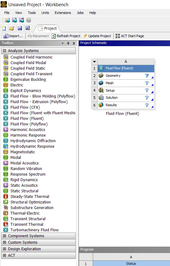
• Now click on geometry to import mixing tee model. It will redirect to Spaceclaim, Ansys’s geometry model.

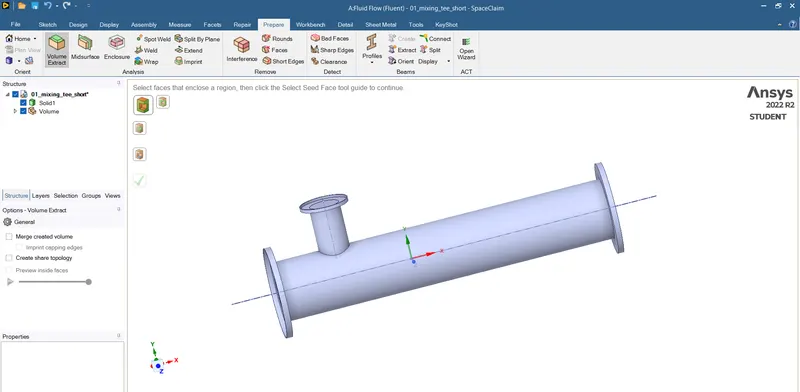
• We are to analyse the mixing of two fluid, so there is role of parts other than two pipes. To supress that we need to extract volume of tee. Go to prepare menu and click on volume extract. Switch to edge selection and select three outer edges and click on green check button.

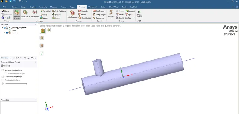
• Hide solid by unchecking it from structure menu to see volume, which we have extracted. Supress solid by clicking on option supress for physics.
• Exit from Spaceclaim and click on mesh to open mesh menu.
• Select outer face and press right click of mouse, it will open a menu. Click on option create named selection and write suitable name for face.

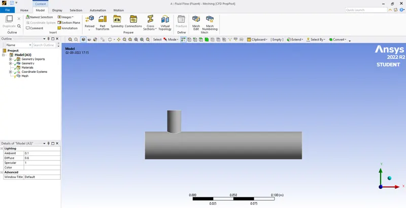
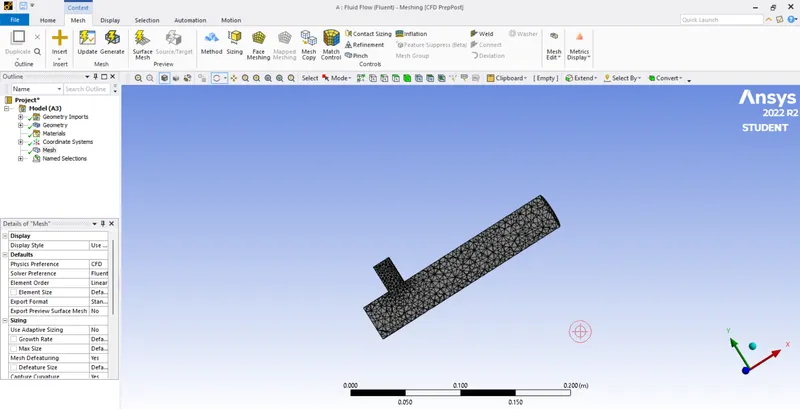
• Now click on mesh option and choose generate mesh. It will generate mesh according to some predefined criteria. Element size can be selected but it is going to affect simulation time. Section plane can be created to see inner portion of geometry.

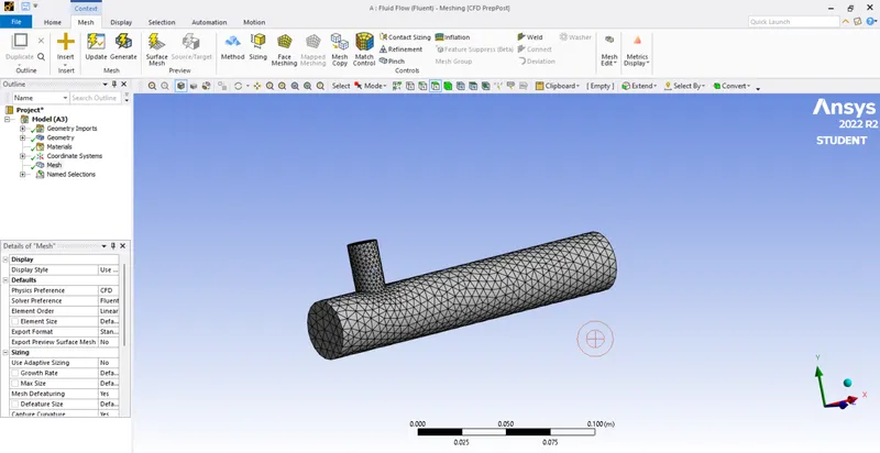
• Cut the plane by using the section plane option and cut half of the portion in the middle to see the inner part of the give model.

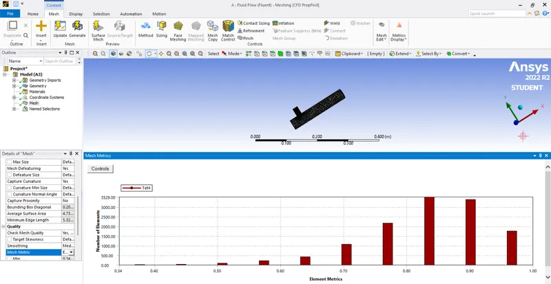
• Select the option element quality to see, how many elements are defying quality. Quality is measured on the scale of 0 to 1. In our graph most of the element are near to 1 so we can say it is good quality.

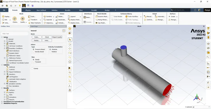
• Exit mesh and open setup. First, Check mesh, it is throwing no error then only we can proceed further. We are going to do pressure based steady state simulation, so choose these options on task page. The part is loaded in the setup module to do the further process.

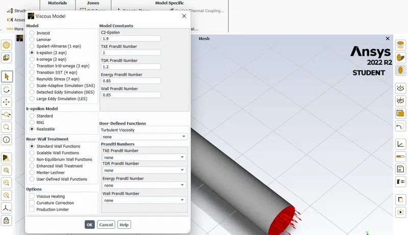
• Go to physics menu and select viscous model. It will open a menu, choose realizable k-epsilon model and close it.

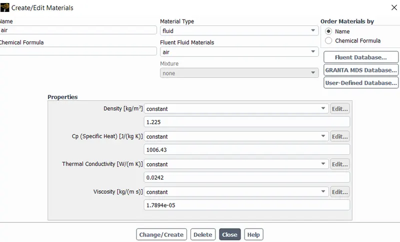
• Click on material and choose air as working fluid. Check working fluid by clicking on cell zone conditions option, if it is air then proceed.

• Now go to boundaries option to set boundary conditions. Select inlet_x and click on option edit. It will open a menu, where all the parameter can be set whether it is thermal, radiation, momentum etc. Put the value of velocity as 3m/s and go to thermal parameter to set temperature as 36C, for hot fluid.

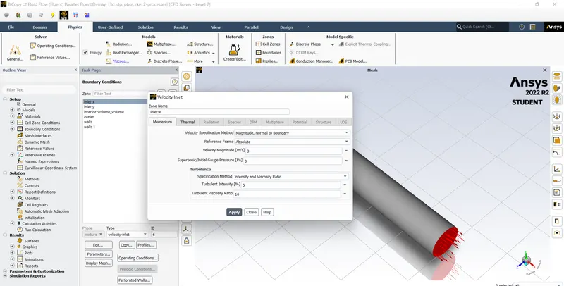
• Repeat the same procedure for cold fluid coming, velocity –6 m/s, temperature – 19C.
• We want to generate temperature report of outlet and we want standard deviation of temperature also. Go to solutions tab and select definition and select area weighted average. In the opened menu select temperature as field variable. Similarly select standard deviation in definitions menu.
• Now click on initialization to calculate approximate values of velocity and pressure.
• Before running the program our final step will be to initialize the problem setup.
• Initialization creates the initial solution that the solver will iteratively improve. Generally, the same converged solution is reached whatever the initialization, though convergence is easier if they are similar. Basic initialization imposes the same values in all cells. You can improve on this in various ways - for example, by patching different values into different zones. Several features, including patching and post-processing, are not available until after initialization.
• The hybrid Initialization method is an efficient method of initializing the solution based purely on the setup of the simulation with no extra information required. These methods produce a velocity field that conforms to complex domain geometries and a pressure field that conforms to complex domain geometries and a pressure field that smoothly connects high and low-pressure values.

SHORT TEE (MOMENTUM RATIO = 2 and HOT INLET VELOCITY = 3m/s)

	K-EPSILON	K-OMEGA
SOLVER TYPE	pressure based	pressure based
VELOCITY FORMULATION	absolute	absolute
TIME	steady	steady
VISCOUS MODEL	realized k-epsilon with standard wall function	k-omega SST model
MATERIAL	air	air
CELL ZONES	inlet-x(velocity inlet) velocity magnitude 3m/s temperature 36C inlet-y(velocity inlet) velocity magnitude 6m/s temperature 19C	inlet-x(velocity inlet) velocity magnite 3m/s temperature 36C inlet-y(velocity inlet) velocity magnitude 6m/s temperature 19C
BOUNDARIES	gauge pressure 0 pa walls = stationary walls	gauge pressure 0 pa walls = stationary walls

SHORT TEE (MOMENTUM RATIO = 4 and HOT INLET VELOCITY = 3m/s)

	K-EPSILON	K-OMEGA
SOLVER TYPE	pressure based	pressure based
VELOCITY FORMULATION	absolute	absolute
TIME	steady	steady
VISCOUS MODEL	realized k-epsilon with standard wall function	realized k-epsilon with standard wall function
MATERIAL	air	air
CELL ZONES	inlet-x(velocity inlet) velocity magnitude 3m/s temperature 36C inlet-y(velocity inlet) velocity magnitude 12m/s temperature 19C	inlet-x(velocity inlet) velocity magnitude 3m/s temperature 36C inlet-y(velocity inlet) velocity magnitude 12m/s temperature 19C
BOUNDARIES	gauge pressure 0 pa walls = stationary walls	gauge pressure 0 pa walls = stationary walls

CASE 1.1:

• Short mixing tee with a hot inlet velocity of 3m/s
• Momentum ratio of 2
• K-Epsilon

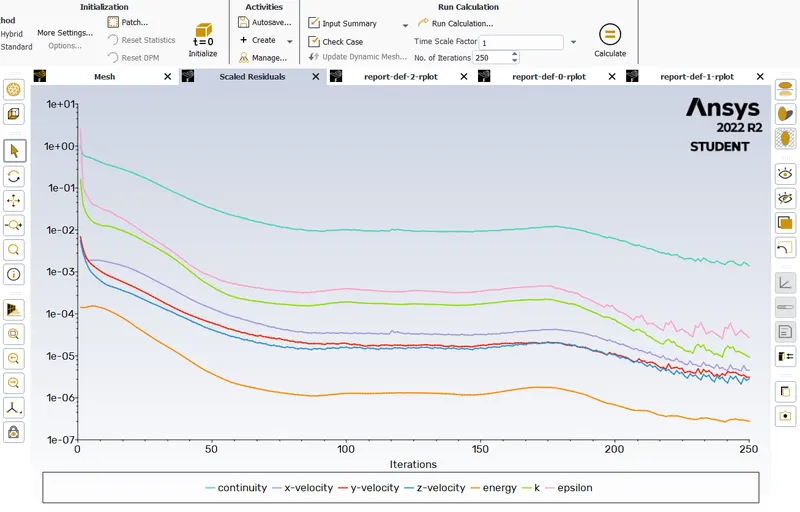
RESIDUAL PLOT :

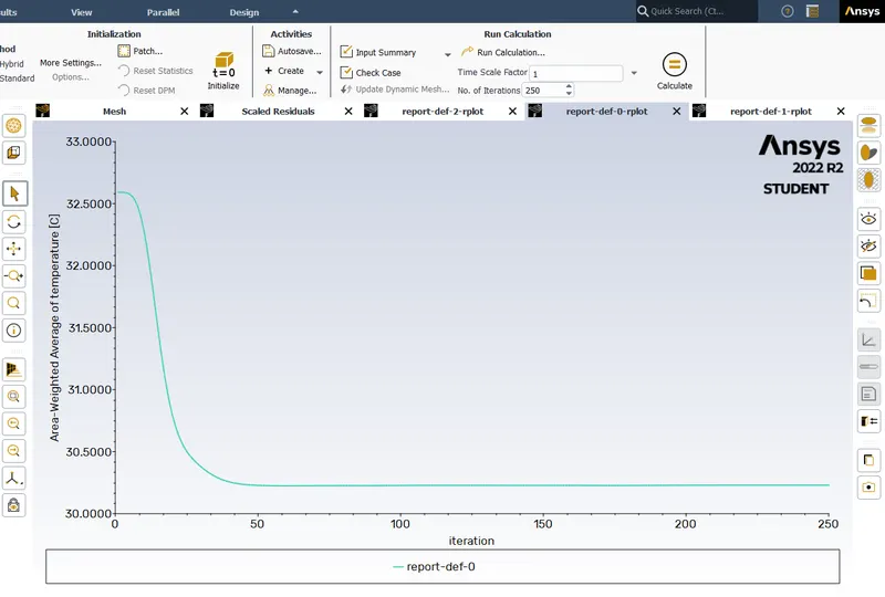
AREA WEIGHTED TEMPERATURE PLOT :

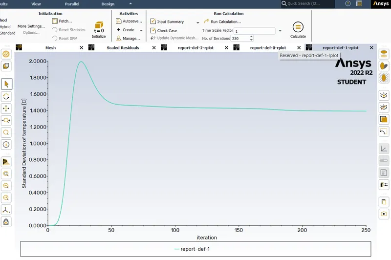
STANDARD DEVIATION OF TEMPERATURE PLOT :

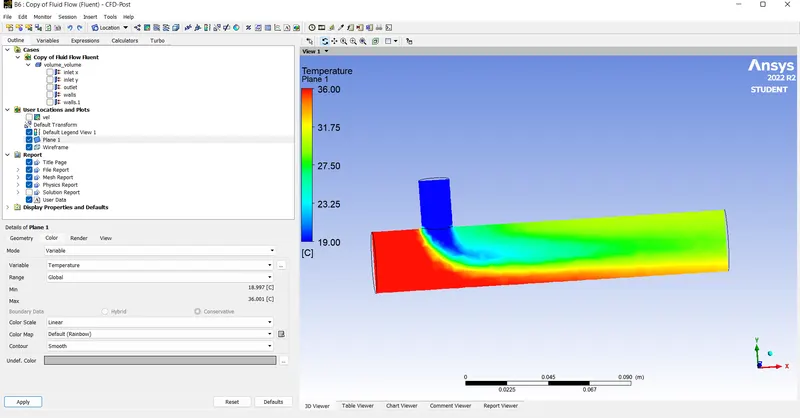
TEMPERATURE CONTOUR :

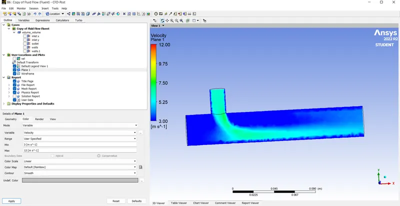
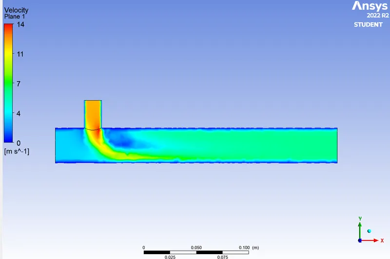
VELOCITY CONTOUR :

CASE 1.2:

• Short mixing tee with a hot inlet velocity of 3m/s
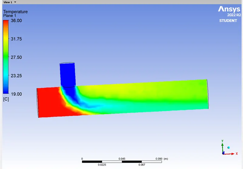
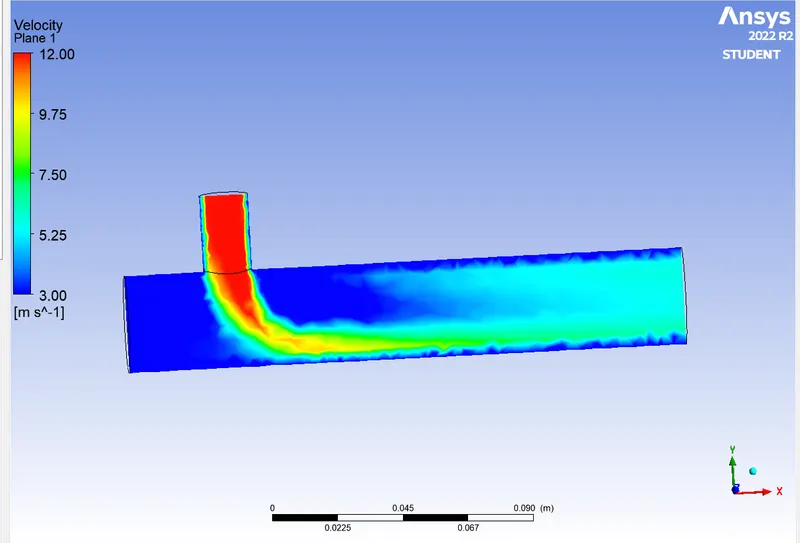
• Momentum ratio of 4
• K-Epsilon

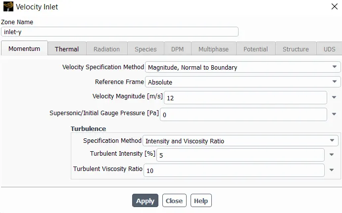
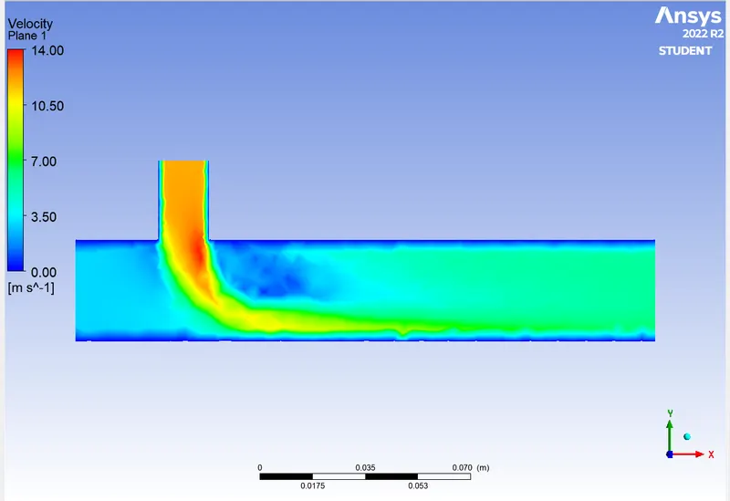
For the momentum ratio of 4 and the inlet velocity of 3, we get the velocity magnitude as 12m/s.

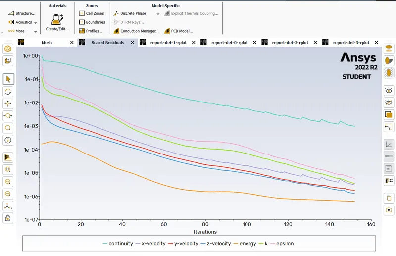
RESIDUAL PLOT :

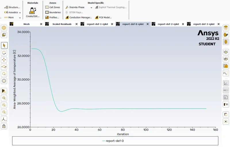
AVERAGE WEIGHTED OF TEMPERATURE PLOT :

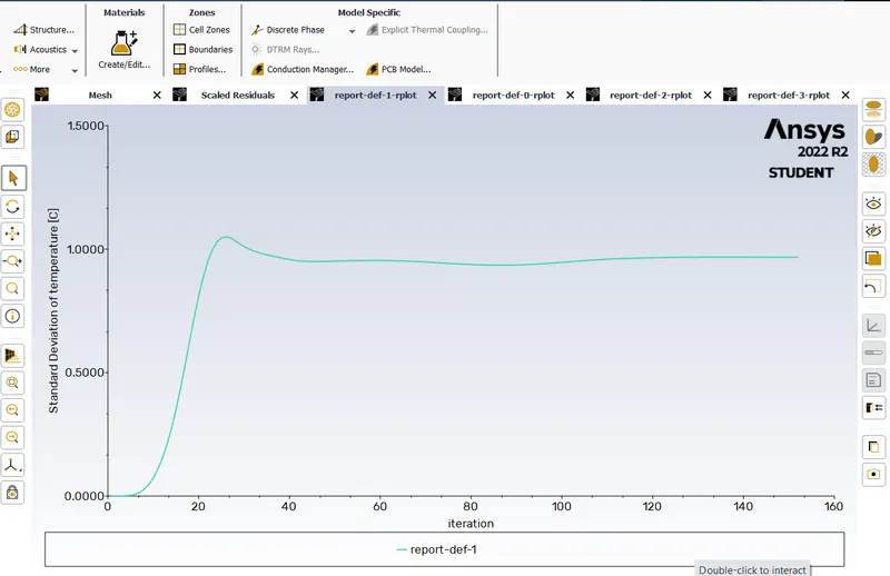
STANDARD DEVIATION OF TEMPERATURE PLOT :

TEMPERATURE CONTOUR PLOT :

VELOCITY CONTOUR PLOT :

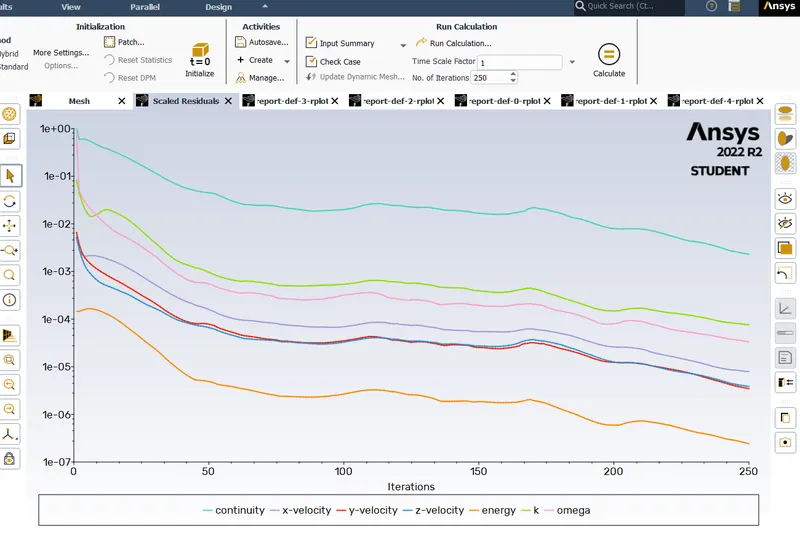
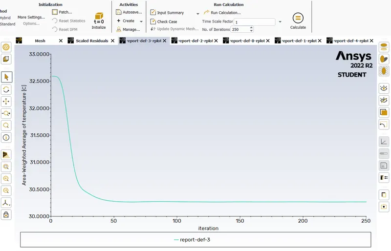
CASE 1.3:

• Short mixing tee with a hot inlet velocity of 3m/s
• Momentum ratio of 2
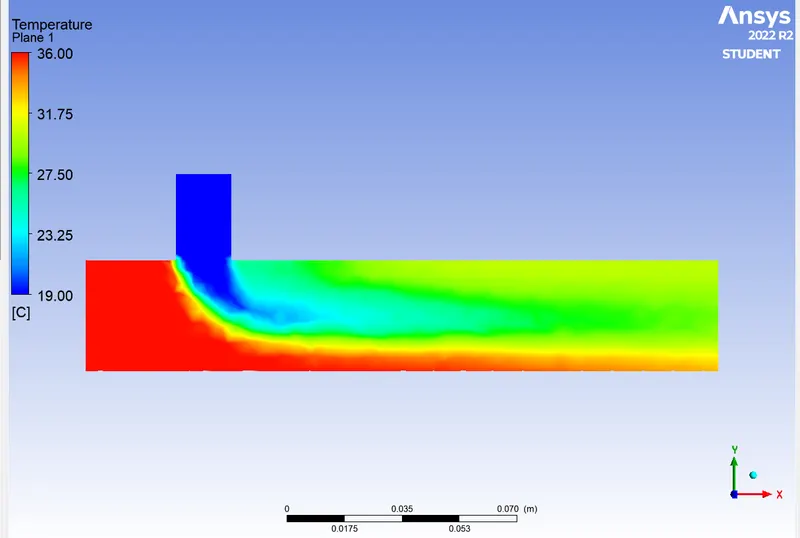
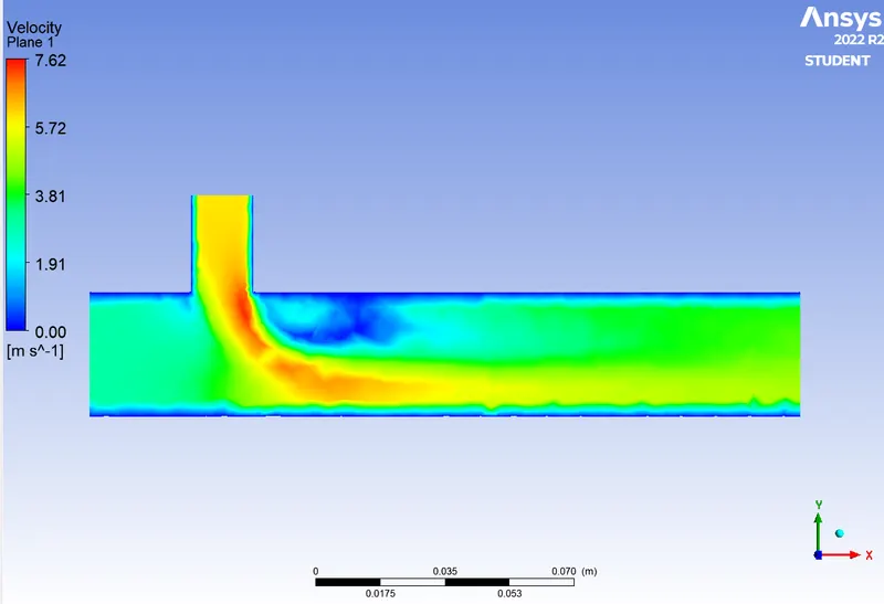
• K-Omega

RESIDUAL PLOT :

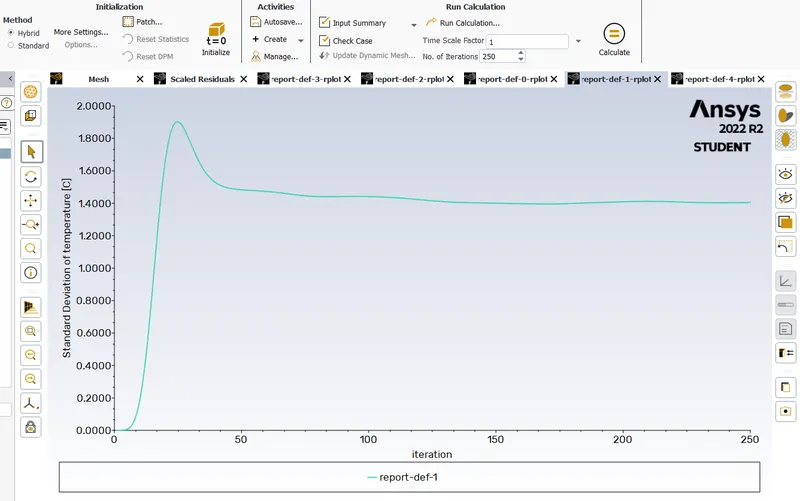
AVERAGE WEIGHTD OF TEMPERATURE PLOT :

STANDARD DEVIATION OF TEMPERATURE PLOT :

TEMPERATURE CONTOUR :

VELOCITY CONTOUR :

CASE 1.4:

• Short mixing tee with a hot inlet velocity of 3m/s
• Momentum ratio of 4
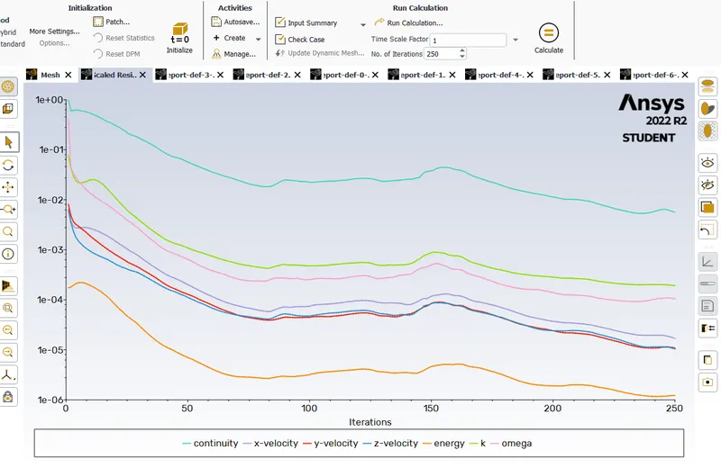
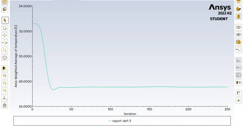
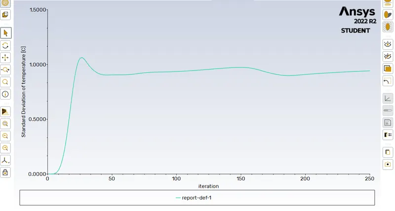
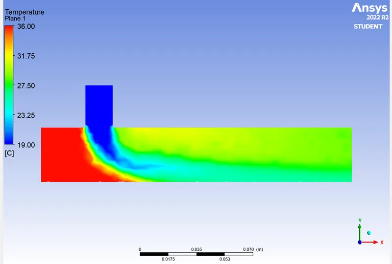
• K-Omega

RESIDUAL PLOT :

AREA WEIGHTED TEMPERATURE PLOT :

STANDARD DEVIATION PLOT :

TEMPERATURE CONTOUR :

VELOCITY CONTOUR :

CONCLUSION:

AVERAGE OUTLET TEMPERATURE:

On comparing the both models with analytical solution we got nearly the same results.

ITERATIONS TO CONVERGE:

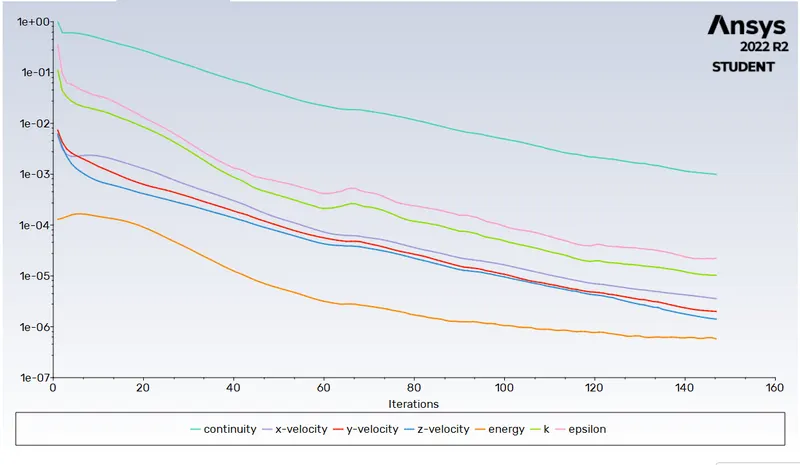
No. of iterations taken to converge is less for Realisable K-epsilon model than K-omega SST model.

STANDARD DEVIATION:

The standard deviation of k-epsilon model is less than k-omega model which shows the better mixing efficiency in k-epsilon model.

So based on the above observations the K-epsilon turbulence model is predicting the results accurately in less no. of iterations. So we can use realisable k-epsilon model for case 2

CASE 2 :

LONG TEE BY USING K-EPLISON

GEOMETRY SETUP :

• The computational models are uploaded to the Ansys Space Claim as a step file.

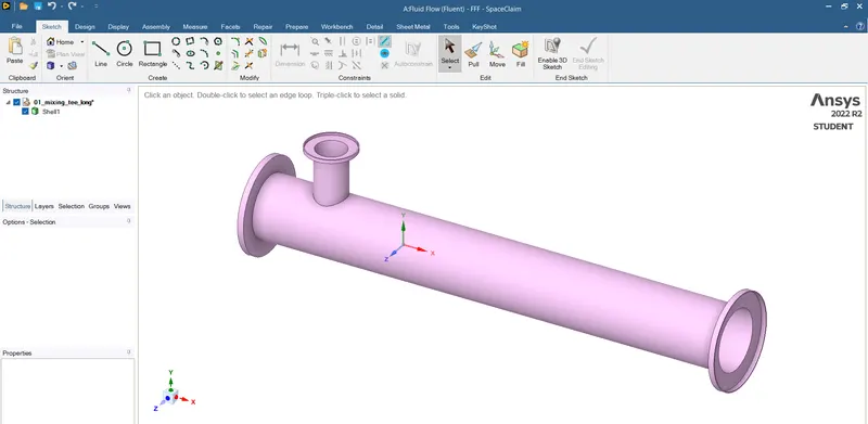
• In this project, we are interested in performing fluid flow analysis through the geometry, hence we used the volume extraction option to extract the fluid volume from the geometry. Then the solid model is suppressed for physics from the fluid model to create mesh at the interested region.

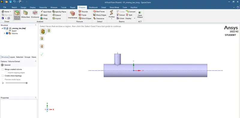
• The boundary names inlet_x, inlet_y, outlet and wall are defined using the named selection option.
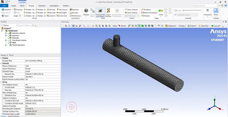
• After generating the mesh, the number of nodes and elements are investigated using the statistics option. Then the mesh quality is checked by choosing the mesh metrices option in quality section.

CASE 2.1 :

LONG TEE (MOMENTUM RATIO=2 and INLET VELOCITY 3m/s)

SETUP	K-EPSILON
SOLVER TYPE	pressure based
VELOCITY FORMULATION	absolute
TIME	steady
VISCOUS MODEL	realizable k-epsilon with standard wall function
MATERIAL	air
CELL ZONES	inlet-x velocity magnitude 3m/s temperature 36C inlet-y velocity magnitude 6m/s temperature 19C
BOUNDARIES	pressure outlet gauge pressure 0 walls - stationary walls

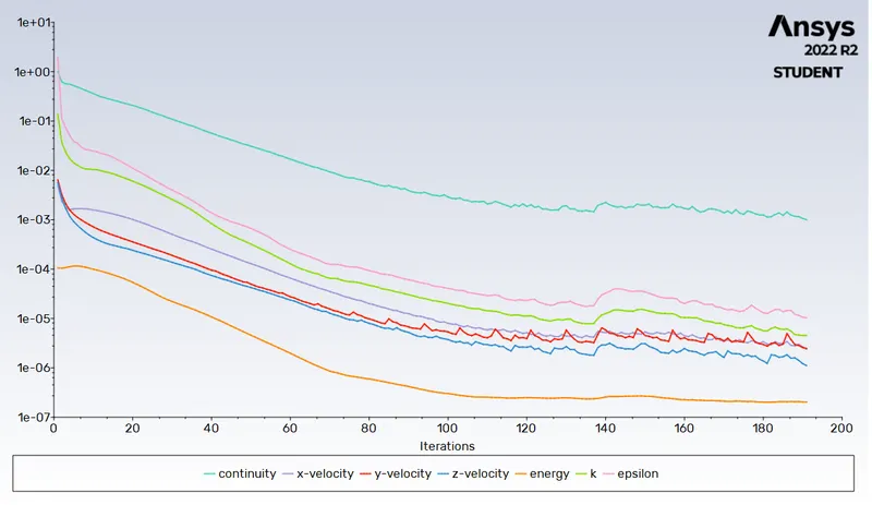
RESIDUAL PLOT :

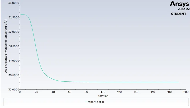
AREA WEIGHTED AVERAGE PLOT :

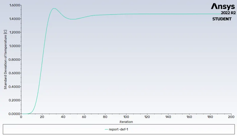
STANDARD DEVIATION PLOT :

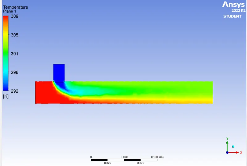
TEMPERATURE CONTOUR :

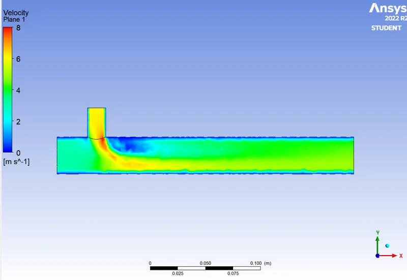
VELOCITY CONTOUR :

CASE 2.2 :

LONG TEE (MOMENTUM RATIO=4 and INLET VELOCITY 3m/s)

SETUP	K-EPSILON
SLOVER TYPE	pressure based
VELOCITY FORMULATION	absolute
TIME	steady
MATERIALS	air
CELL ZONES	inlet-x velocity magnitude 3m/s temperature 36C inlet-y velocity magnitude 12m/s temperature 19C
VISCOUS MODEL	realizable k-eplison with standard wall function
BOUNDARIES	pressure outlet gauge pressure 0 walls - stationary walls

RESIDUAL PLOT :

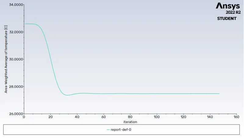
AREA WEIGHTED AVERAGE :

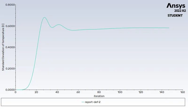
STANDARD DEVIATION :

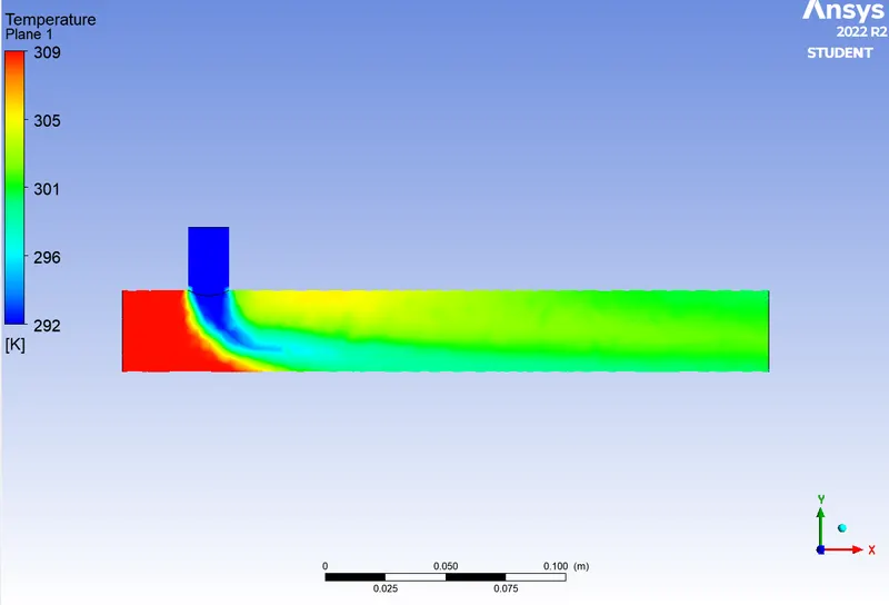
TEMPERATURE CONTOUR :

VELOCITY CONTOUR :

CONCLUSION :

Ansys fluent is high performance CFD software recognized for accuracy, robustness etc. it is not confined to only aerospace and mechanical domain, it has various application like to simulation of calculation of air flow on air craft wing, combustion in furnace, bubble columns in oil refineries, combustion in IC engine etc. In this study we performed simulation on simple geometry of mixing tee and got insights of various feature of fluent. we can conclude by analysing graph that If momentum ratio is increased, outlet temperature will decrease and there is no effect of velocity even though length is increased.

• As seen, the temperature at the outlet drops down significantly due to the high velocity of cold air from the inlet. This is possible due to turbulent mixing at the tee joint between hot air and cold air because of the high velocity of cold air, which is not possible in the case of low-velocity cold air.
• The temperature contour at the outlet for short tee cases shows that some of the high-temperature flow sips through without properly mixing with the flow. Whereas, in the temperature contour of long tee cases, the high temperatures flow thoroughly mixes with the rest of the flow.
• Therefore, we can recommend using the long tee and high-velocity inlet for application. This is because we have a low standard derivation in the case of long tee compared to the short tee for both momentum ratios.
• K-epsilon model predicts well far from boundaries (wall) and K- omega model predicts well near the wall. Even though it depends on Y+. Therefore, the K-epsilon model is majority used for free flow away from the wall and as in this project, there is no dealing with the wall of the mixing tee for change in temperature along the length of it, so the K-epsilon model was chosen for further simulations.