Week 1- Mixing Tee

AIM:

For two versions of the mixing tee (long & short) set up steady-state simulations to compare the mixing effectiveness when hot inlet temperature is 36⁰C & the Cold inlet is at 19⁰C using the k-epsilon and k-omega SST model for the first case and use the more suitable model for further cases. Give the reason for choosing a suitable model.

1. Case 1
   • Short mixing tee with a hot inlet velocity of 3m/s.
   • Momentum ratio of 2, 4.
2. Case 2
   • Long mixing tee with a hot inlet velocity of 3m/s.
   • Momentum ratio of 2, 4.

Momentum ratio = velocity at cold inlet / velocity at hot inlet

In a table, compare the following values from the 2 cases.

1. Cell count
2. Average outlet temperature
3. Number of iterations for convergence

EXPECTED RESULT:

1. Velocity and temperature contour plots on the cut planes along and across the pipe.
2. Velocity and temperature line plots along and across the length of the pipe.
3. Perform Mesh independent study for any one case.
4. Discuss the effect of length and momentum ratio on results.

DESCRIPTION:

CFD is a branch of fluid mechanics, which uses mathematics, physics and computational software to visualize how fluid flows and affects its medium and its neighbours.In CFD mostly computers are used to predict the fluid flow phenomena based on some governing equations like conservation of momentum, Navier stokes equation, conservation of energy etc.In this study we are going to simulate the effect of fluid using Ansys fluent software.Ansys fluent is an important tool in CAE domain, which allows you to perform all the three major steps of any simulation pre-processing, solving and post-processing.Ansys fluent facilitates for modelling flow, turbulence, heat transfer and chemical reactions.

Mixing tee is a device which uses specifically engineered internal geometry to mix two fluid streams into one stream, efficiently.In this study we are going to find the effectiveness of mixing tee.Hot air and cold air are going to be mixed in mixing tee.They will have different veclocities.We will use two different mixing tee distinguished with length and analyse the effect over length on mixing.

PROCEDURE:

1.Understand and define the problem statement for each case.

2.Open Ansys workbench and set up a fluent simulation setup and rename it accrodingly.

3.For fluent setup, open space claims and load the geometry.Extract the working fluid region from the loaded geometry to compute simulation in that particular region.And then close space claim.

4.Next in mesh setup, provide boundary names for each surface and generate mesh to the fluid flow volume.Close mesh setup and update the mesh.

5.Later in the setup section provide all the required parameters accroding to the simulation, such as simulation type, input velocity and temperature, materials (working fluid) and other user defined parameters.

6.In set up parameters understand the concept of k-epsilon and k-omega SST and find out which is convenient for the curren simulation.

7.Then simulate the problem set up for the number of iteration required to converge the results.

8.Then close and update the setup.Open the results section to see all the simulated results.

9.Compare generated results from each case for their cell count, average outlet temperature and number of iteration for convergence.

10.Display contour plot on the cut plane to visualize velocity and temperature distribution along and across the mixing tee's length.

11.For a more detail examination, plot velocity and temperature line chart along the mixing tee's length.

12.Validate the test by performing a mesh independence study on any one case.

13.Study the effect of length and momentum ration on the results of each case.

14.Plot the convergence graph to verify that all the results are fully converged after running numerous iterations.

SET UP CASES FOR MIXING TEE

To understand k-epsilon and k-omega SST for case-I for simulation of turbulence modeling where k-epsilon models predict flow virtually far from wall (boundaries) and k-omega model predicts near the wall.

Case-I Short Mixing Tee

1.Simulation-1: Hot inlet velocity 3m/s Momentum ratio 4

2.Simulation-II: Hot inlet velocity 3m/s Momentum ratio 2

Case-II Long Mixing Tee

1.Simulation-III: Hot inlet velocity 3m/s Momentum ratio 4

2.Simulation-IV: Hot inlet velocity 3m/s Momentum ratio 2

SIMULATION-I: SHORT MIXING TEE (Hot inlet velocity 3m/s Momentum ratio 4)

For the 1st case we set two setups, one for k-epsilon and another for k-omega SST but we use same geometry and mesh for both cases of simulation.

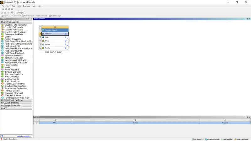
Firstly we open the Ansys Workbench and pull the Fluid dlow(fluent) to the work space project and double click on geometry to open the Ansys spaceclaim, on the extreme left corner it shows starting space claim

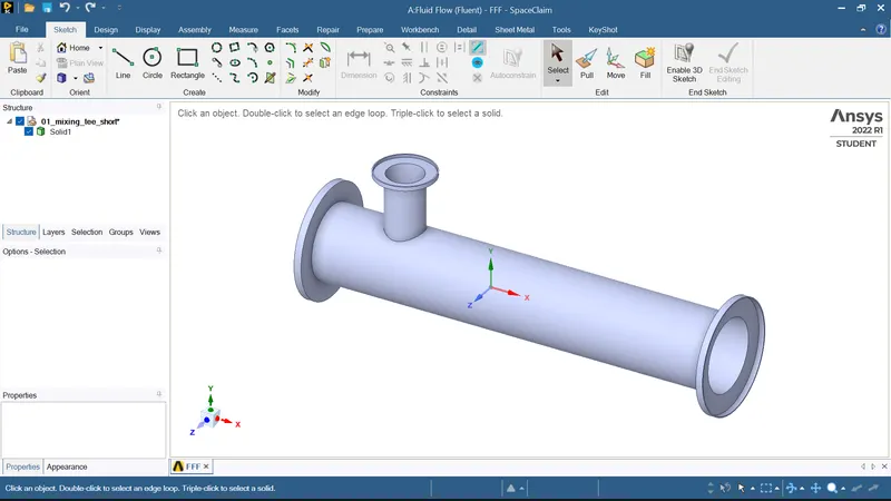
SPACE CLAIM:

Then opening the short mixing tee model in space claim as follows

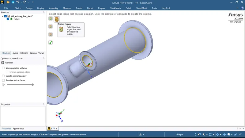
As we are interested in only the fluid flow internally we go to prepare options and select volume extract and then select edges and remove the edges we are not concerned with and click on arrow tick as follows

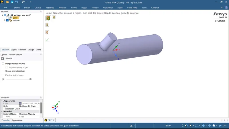
And now deselct the solid model and select supress for physics are the solid model only loads during meshing as follows and close the space claim it automatically gets saved

MESHING:

Now opening the meshing the model file of space claim opens here as follows

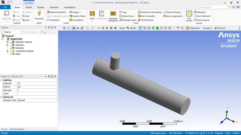
Now selecting the edge face option and naming them as follows

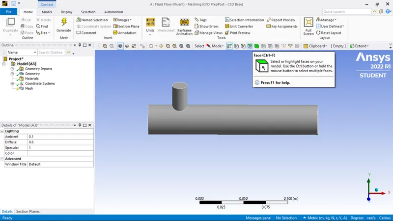
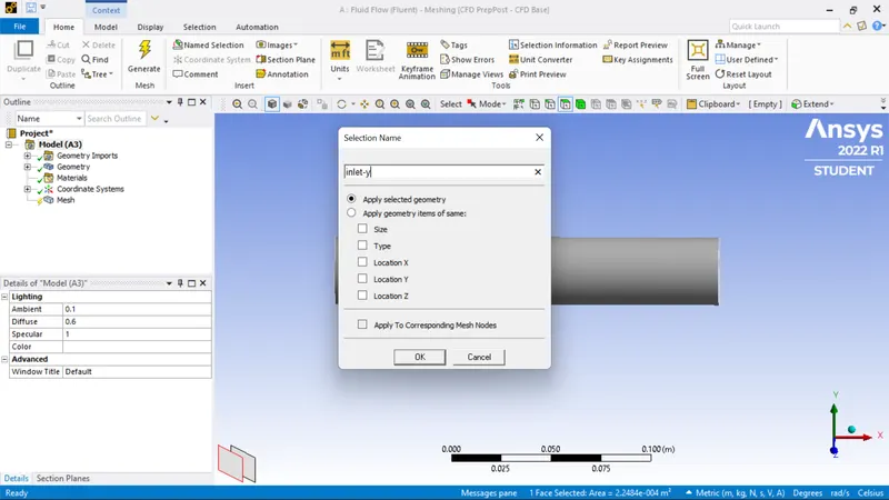
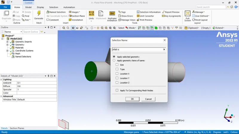
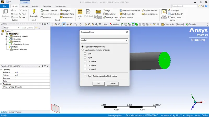
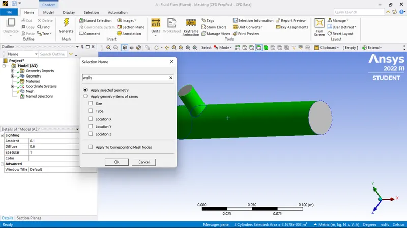
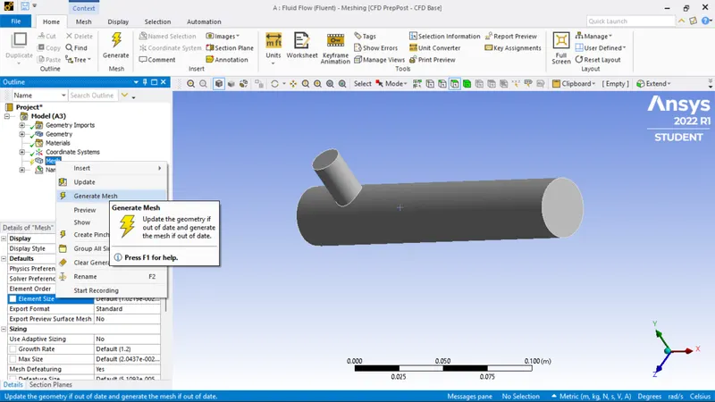
On clicking generate mesh we get as follows mesh by default

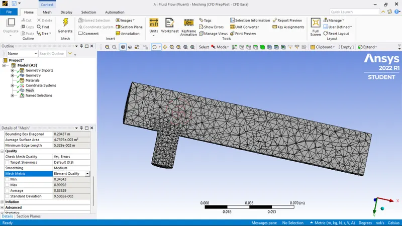
Selecting the quality with element quality for mesh metric we get as follows

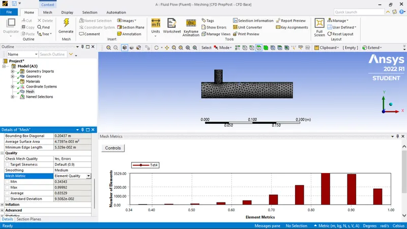
Cutting along plane Y to check the mesh geometry

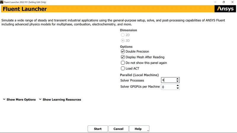
FLUENT LAUNCHER:

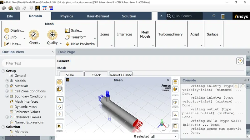
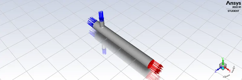
The model file in fluent looks are follows with inlets and outlets

Checking the mesh quality for it is suitable for fluent analysis or not so if not to improve the quality.

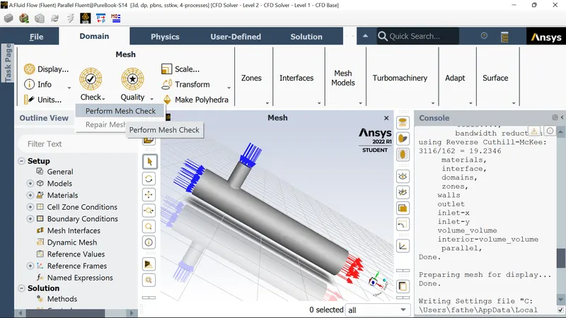
It prints the following and mesh is suitable.

Domain Extents:
   x-coordinate: min (m) = -7.733225e-02, max (m) = 1.150456e-01
   y-coordinate: min (m) = -1.693636e-02, max (m) = 4.316116e-02
   z-coordinate: min (m) = -1.693804e-02, max (m) = 1.693801e-02
 Volume statistics:
   minimum volume (m3): 7.709761e-10
   maximum volume (m3): 6.709235e-08
     total volume (m3): 1.773828e-04
 Face area statistics:
   minimum face area (m2): 1.556574e-06
   maximum face area (m2): 3.452893e-05
 Checking mesh.....................................
Done.
 

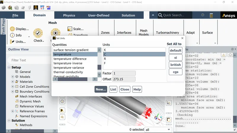
Now setting up the units for temperature

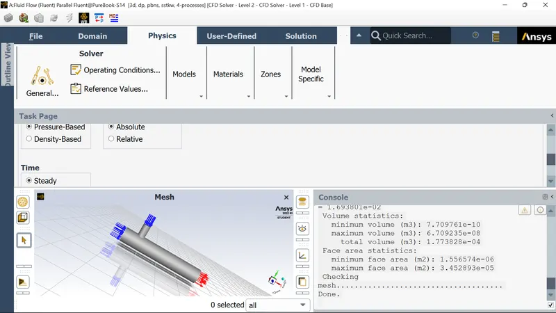
Then setting up the physics of the domain.Keeping the general parameter setting as it is. Solver type=pressure based; velocity formulation=Absolute; Solver time=steady.

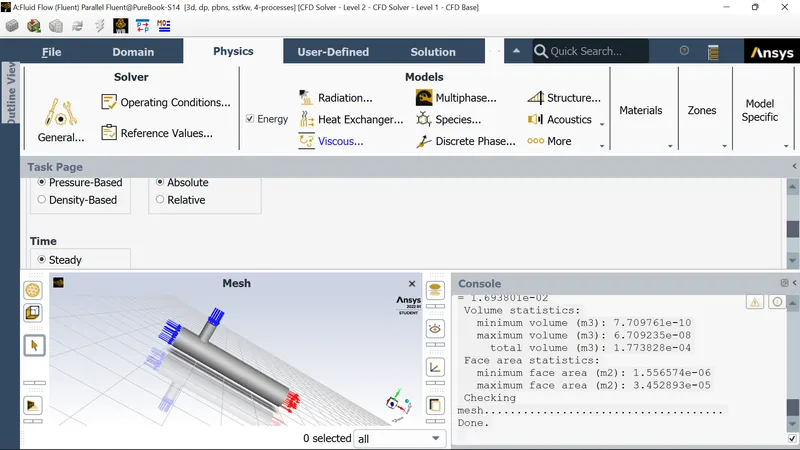
Now activate the model by turning the energy equation. Activating energy equation allows the temperature-dependent problem to be solved.

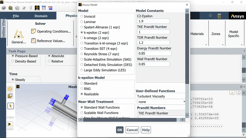
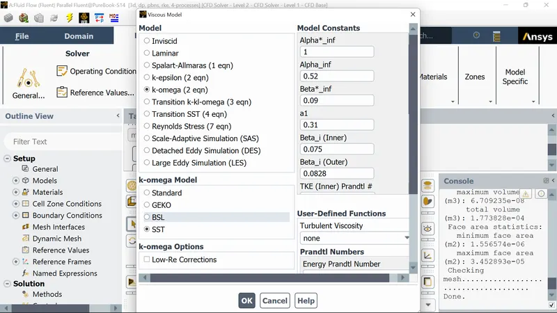
Then in the viscous model, delect 'k-epsilon',Realizable for our first type of simulation.

In materials in case our working fluid is air so we keep the default material if not we would click the 'fluent database' and add new material.

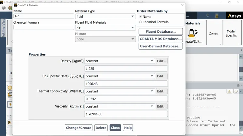
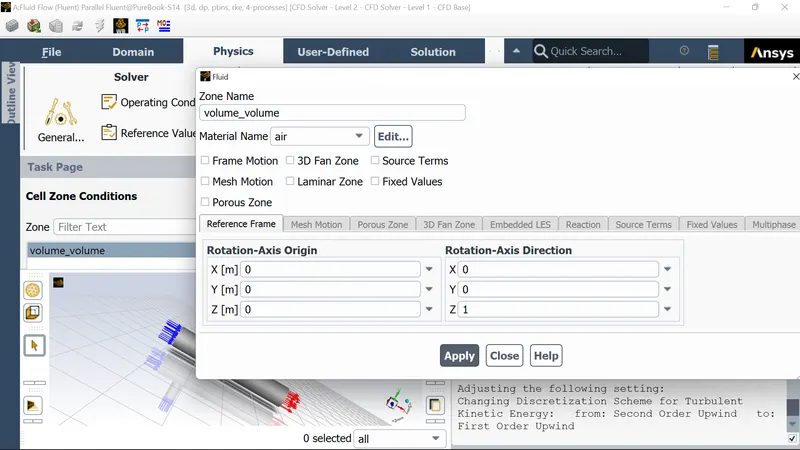
Next in the cell zone define the material type, select the working fluid (air). Here its set to air already.

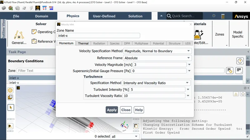
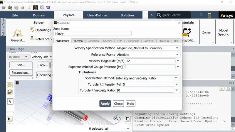
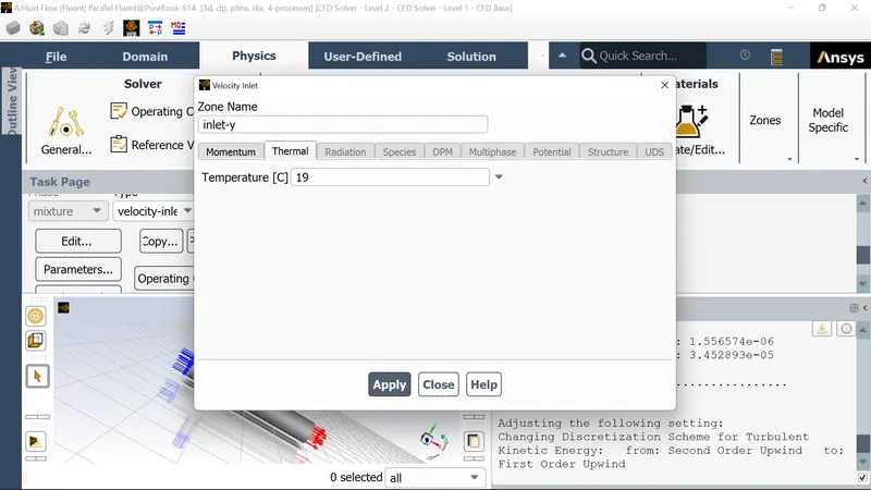
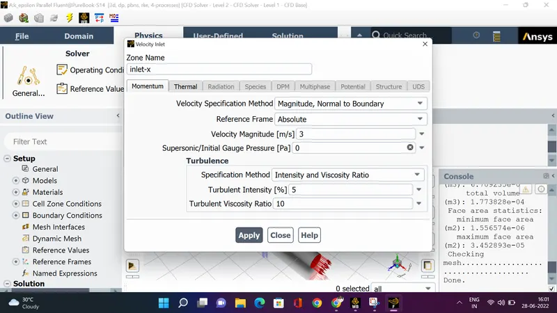
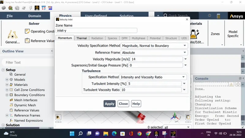
And in Boundary conditions select inlet-x and define inlet velocit as 3m/s and temperature as 36 celcius. For inlet-y setting velocity as 12m/s (sincemomentum ratio 4) and temperature as 19celcius.

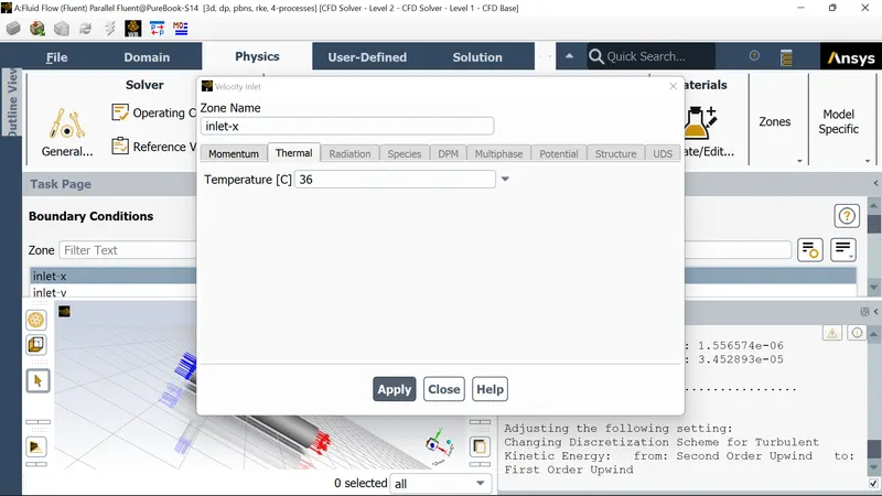
For inlet-y cold air

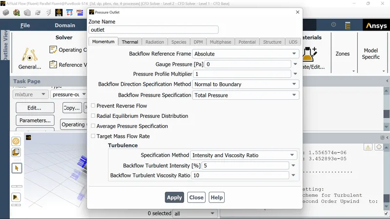
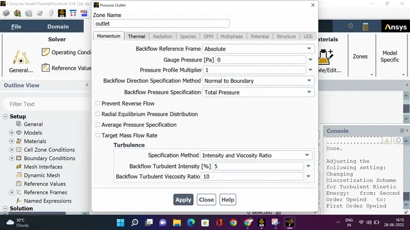
For outlet, pressure condition of atmospheric pressure value which is also zero gauge pressure.The backflow will bring turbulence and energy back into the model.It is therefore necessary to specify the backflow conditions.

Next in the solution section in reports select area weighted average as follows

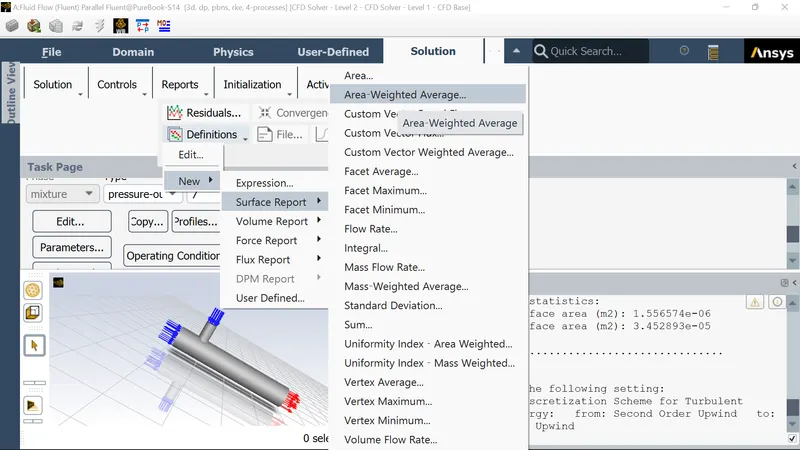
Here for temperature average at outlet surface we need report so selecting temperature and check for report file and report plot as follows

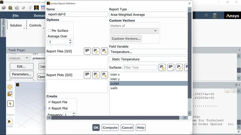
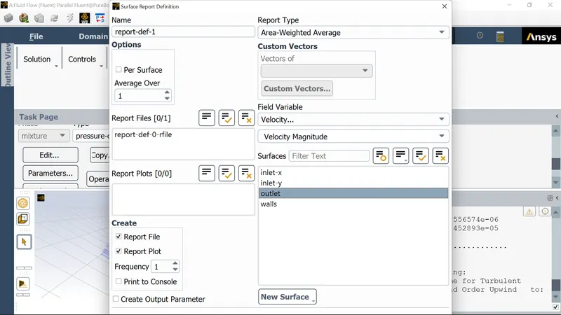
Similarly creating the plot for average velocity plot at out let boundary condition as follows

Now, final step is to initialize the problem setup.

The hybrid initialization method is an efficient method of initializing the solution purely on the setup of the simulation with no extra information required.

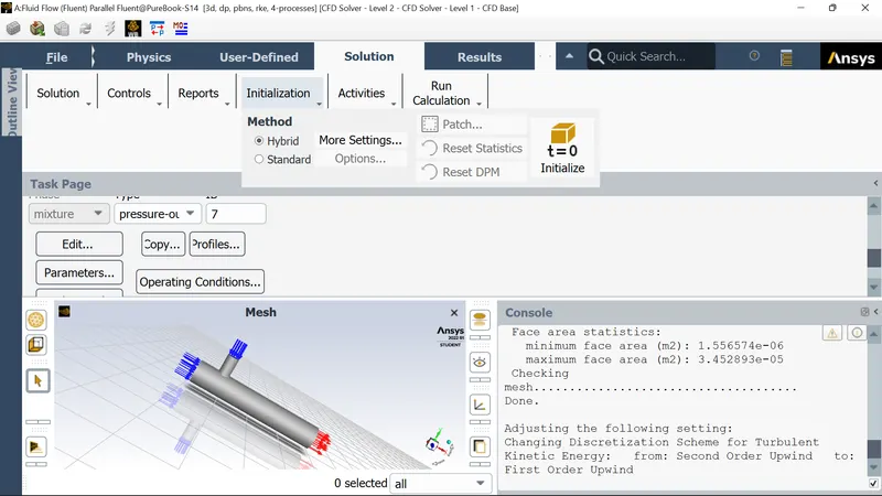
on running the initialization the data printed in the console says initialization is done as follows.

Initialize using the hybrid initialization method.

Checking case topology... 
-This case has both inlets & outlets 
-Pressure information is not available at the boundaries.
 Case will be initialized with constant pressure

	iter		scalar-0

	1		1.000000e+00
	2		1.276574e-03
	3		2.033570e-04
	4		4.417501e-05
	5		3.802115e-05
	6		1.639359e-05
	7		3.955840e-05
	8		7.481948e-06
	9		1.450585e-05
	10		3.022394e-06

Hybrid initialization is done.

Warning: convergence tolerance of 1.000000e-06 not reached
during Hybrid Initialization.

Now we run the simulation by entering no of iterations for which we want the simulation and press calculate.

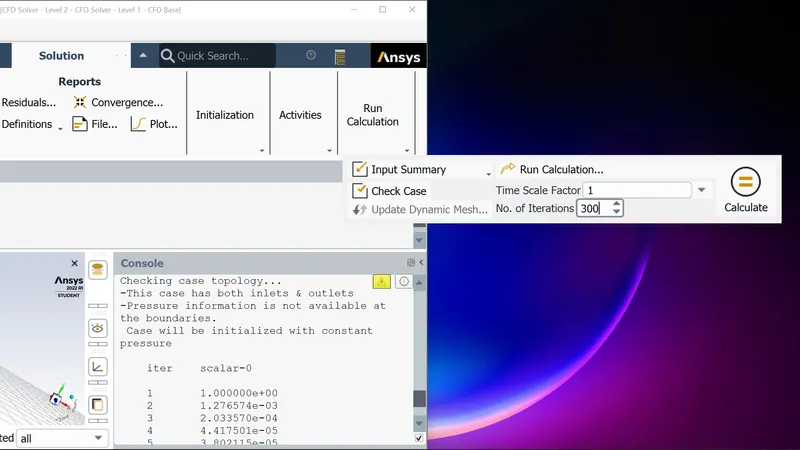
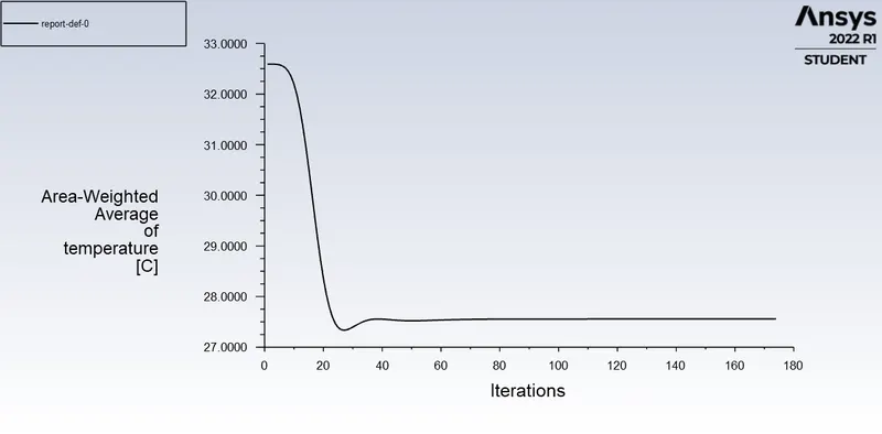
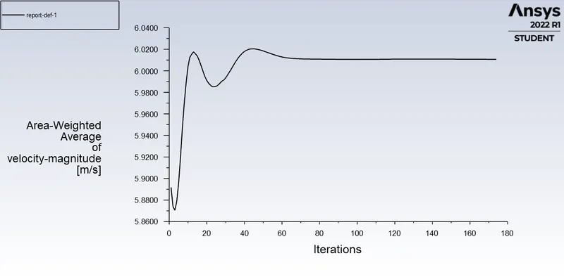
When the solution is fully converged it will show the following the console and the plots are plotted as follows

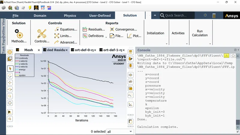
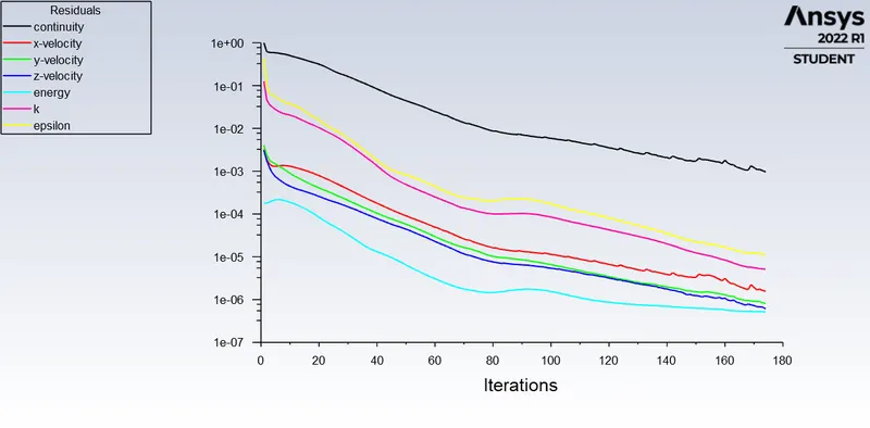
For temperature at outlet

For velocity at outlet

After this close the fluent and post-process the results.Click on results in workbench and it will open CFD post.

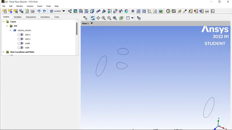
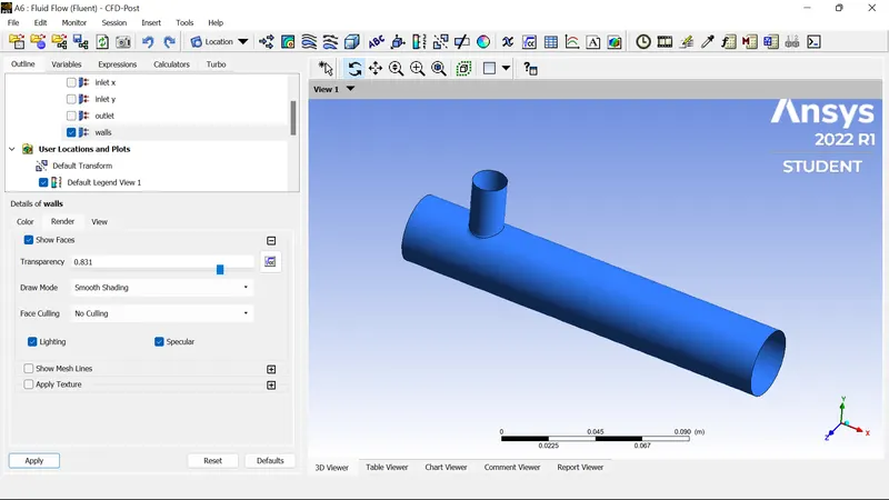
selecting only the walls and rendering

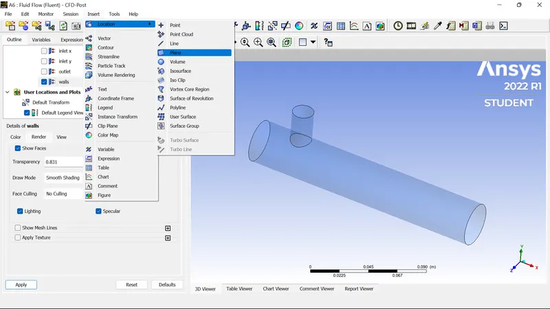
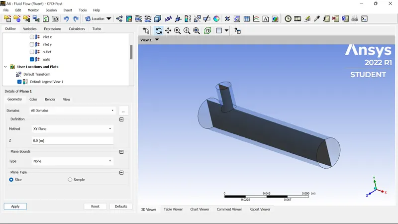
creating the xy plane in the model to look for the temperature and velocity contour

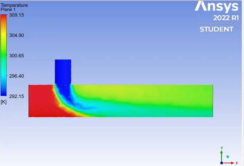
Giving the range from 19 to 36 celcius

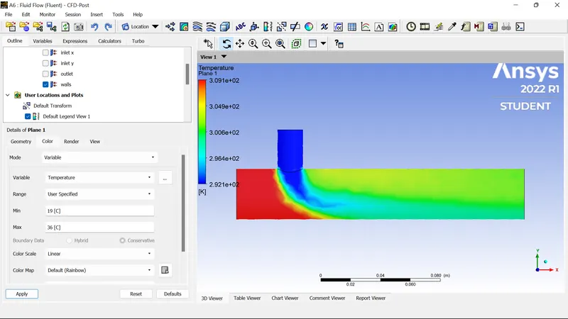
For temperature

For velocity

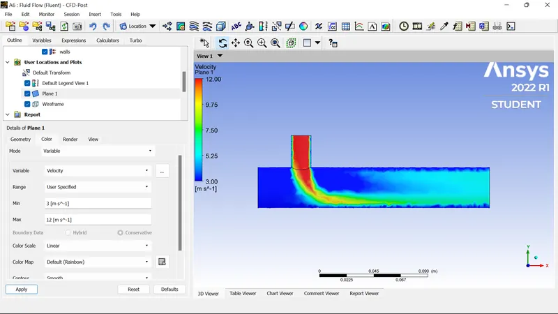
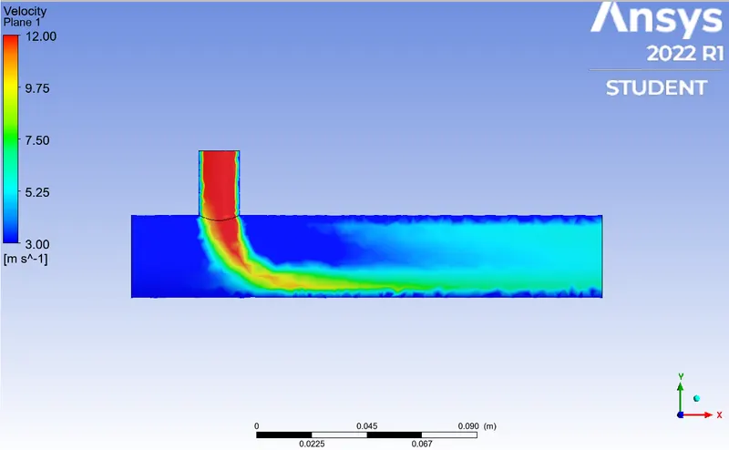
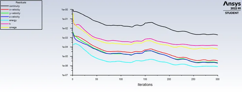
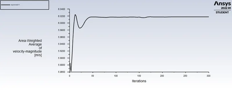
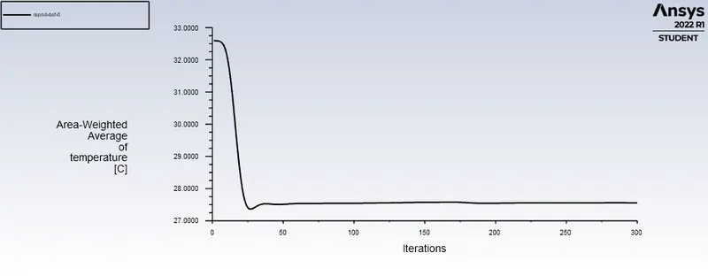
Now similarly doing for k-omega SST

Residual plots

Area weighted average for velocity

Area weighted average for temperature

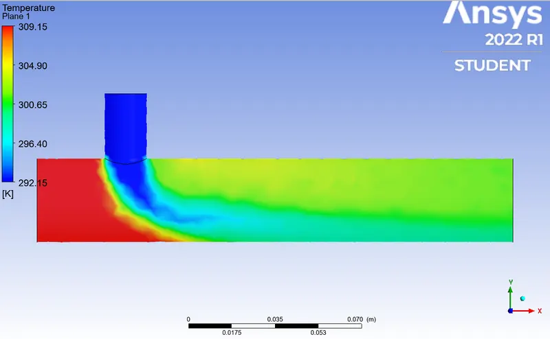
For temperature contour

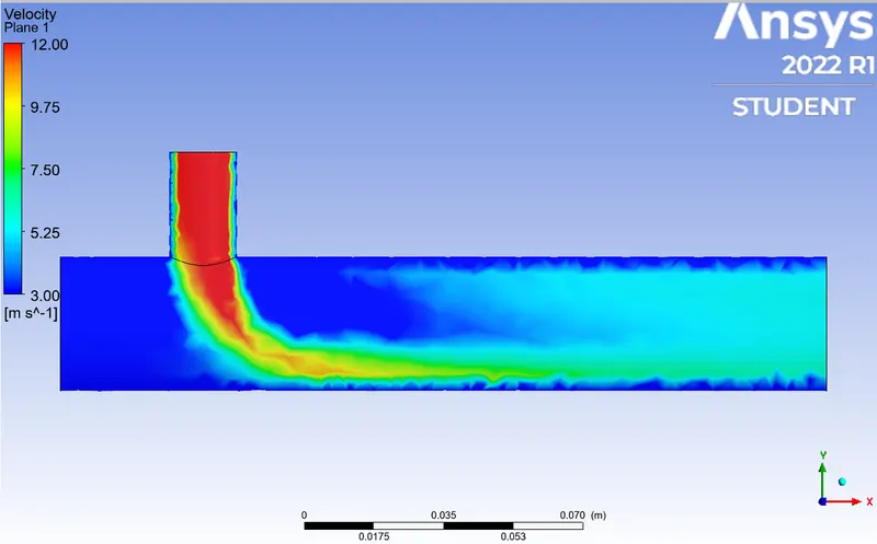
For velocity contour

K-EPSILON

K-epsilon turbulence model is the most common model used in CFD to simulate the mean flow characteristics for turbulent flow conditions.It is a two equation model that gives a description of turbulence by means of two transport equations (PDEs), the first transported variables are the turbulent kinetic energy k and the second transported variable is the rate of dissipation of turbulent kinetic energy.

K-epsilon focuses on the mechanism that affecrs the turbulent kinetic energy.

K-OMEGA SST

The K-Omega SST turbulence model is two equation eddy viscosity model that is used for many aerodynamic applications.It is a hybrid model combining the Wilcox k-omega and k-epsilon models.A blending function F1 activates the wilcox model near the wall and the k-epsilon model in the free stream.This ensures that the appropriate model is utilized through the flow fluid.

DIFFERENCE B/W K-EPSILON AND K-OMEGA

The k-omega model is well suited for simulating flow in the viscous sub-layer.On the contarary k-epsilon this is deal for predicting flow in the regions away from the wall.

Here in the above models we see that both the temperature and velocity contour are same as it depends on the meshing size of the elements refinement.

SIMULATION-II: SHORT TEE (Hot inlet velocity 3m/s Momentum ratio 2)

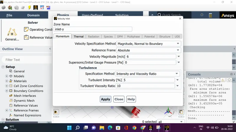
Inlet cold air velocity = 6m/s

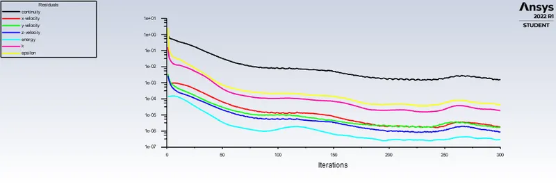
Residual plots

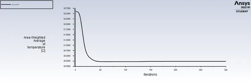
Area weighted average for temperature

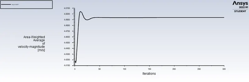
Area weighted average for velocity

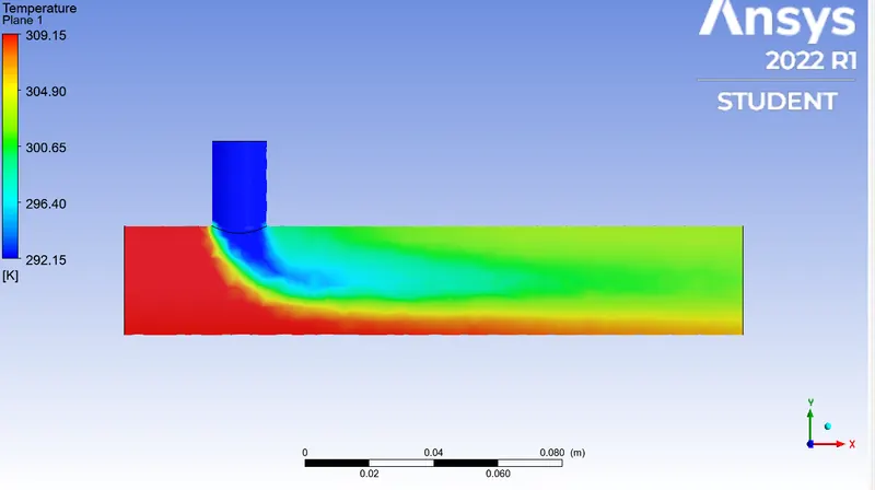
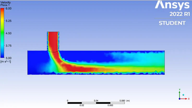
Temperature contour

Velocity contour

CASE-II:

SIMULATION-III: LONG TEE(Hot inlet velocity 3m/s Momentum ratio 4)

Inlet cold air velocity = 12m/s

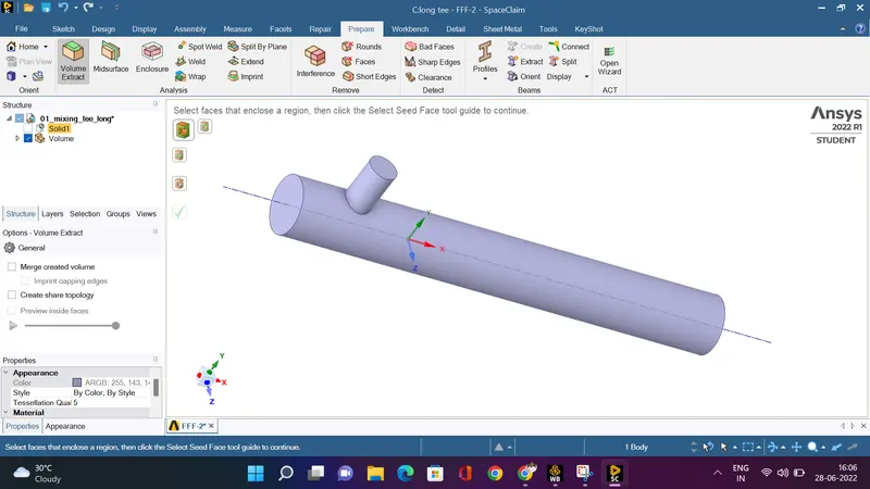
GEOMETRY

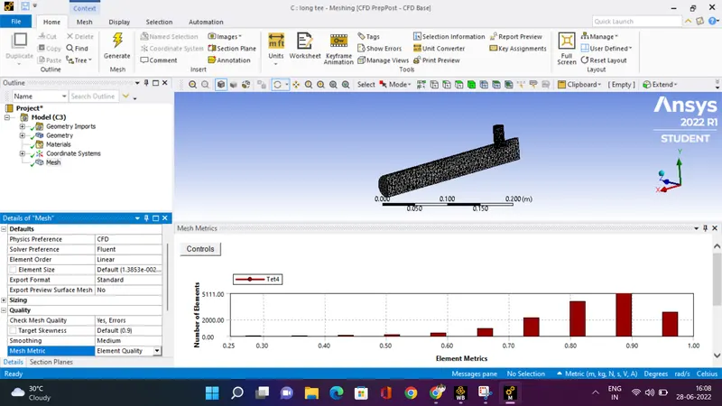
MESHING

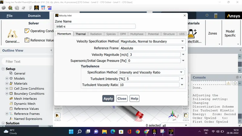
FLUENT

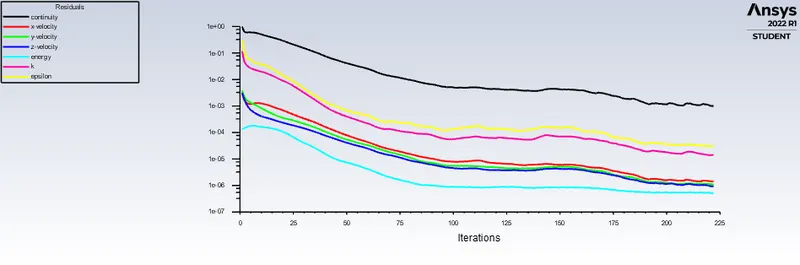
Residual plots

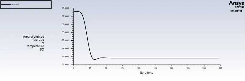
Area weighted average for temperature

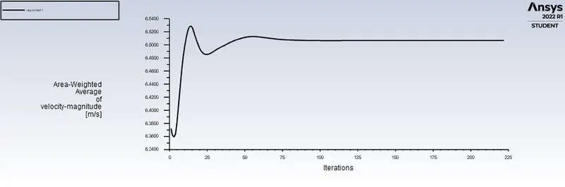
Area weighted average for velocity

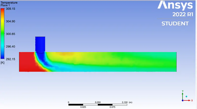
Temperature contour

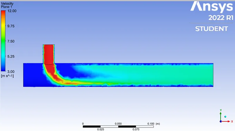
Velocity contour

SIMULATION-IV: LONG TEE (Hot inlet velocity 3m/s Momentum ratio 2)

Inlet cold air velocity = 6m/s

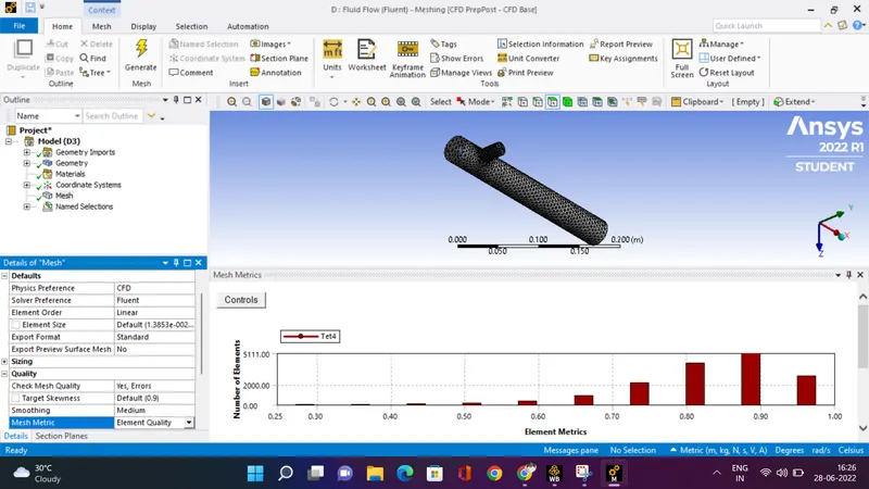
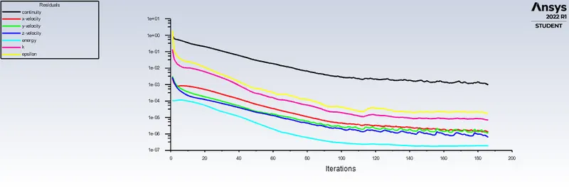
Residual plots

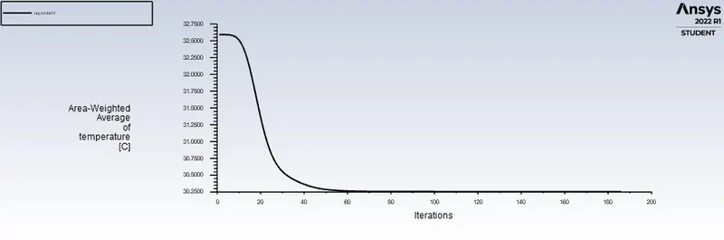
Area weighted average for temperature

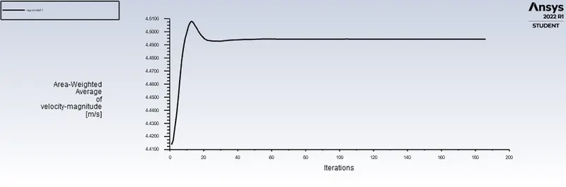
Area weighted average for velocity

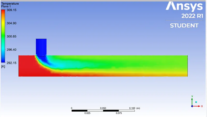
For temperature contour

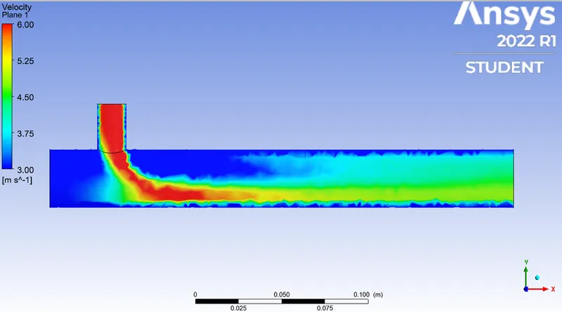
For velocity contour

MESH INDEPENDENCE TEST

This is performed to study and analyze the dependence of the results on the mesh density.

So we will run for one more mesh element size of 0.004 and check the simulation results

For short Mixing tee with momentum =4

ELEMENT SIZE IN m	NO OF ELEMENTS	AVERAGE VELOCITY OF OUTLET m/s	AVERAGE TEMPERATURE AT OUTLET kelvin	NO OF ITERATIONS	MESH INDEPENDENCE
0.012019	3529	4.49	30.25	180	yes
0.004	6126	4.48	30.26	300	yes

So we can see that change in element size doesn't effect the outlet temperature and velocity.

COMPARISION OF RESULTS:

TYPE OF TEE & MOMENTUM	ELEMENT SIZE IN m	NO OF ELEMENTS	AVERAGE VELOCITY OF OUTLET m/s	AVERAGE TEMPERATURE AT OUTLET kelvin	NO OF ITERATIONS
Short tee momentum=4	0.012019	3529	4.49	30.25	180
Short tee momentum=2	0.012019	3529	4.49	30.25	300
Long tee momentum=4	0.012019	5111	6.5	27	225
Long tee momentum=2	0.012019	5111	4.49	30.25	190

CONCLUSION:

Thus we observed that k-epsilon and k-omega doesn't vary for the same mesh size for the temperature and velocity contour for the short tee mixing. And we saw that length of the tee does not affect the results at the output that much if we ignore the diffusion. And all results are mesh independent.