Week 1- Mixing Tee

Aim-

For this challenge, we have created two versions of the mixing tee. One of them is longer than the other.

Your job is to set up steady-state simulations to compare the mixing effectiveness when hot inlet temperature is 36⁰C & the Cold inlet is at 19⁰C.

Use the k-epsilon and k-omega SST model for the first case and based on your judgment use the more suitable model for further cases. Giving the reason for choosing a suitable model is compulsory.

1. Case 1
   • Short mixing tee with a hot inlet velocity of 3m/s.
   • Momentum ratio of 2, 4.
2. Case 2
   • Long mixing tee with a hot inlet velocity of 3m/s.
   • Momentum ratio of 2, 4.

Momentum ratio = velocity at cold inlet / velocity at hot inlet

In a table, compare the following values from the 2 cases.

1. Cell count
2. Average outlet temperature
3. Number of iterations for convergence

Expected results:

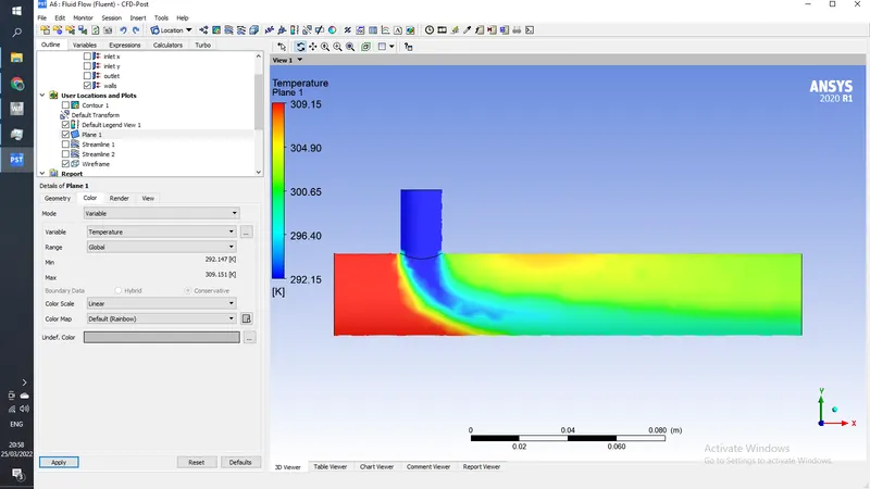
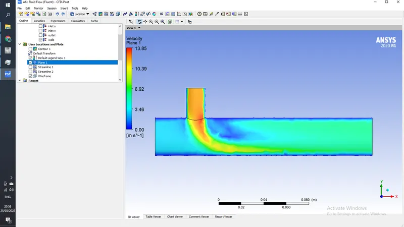
1. Velocity and temperature contour plots on the cut planes along and across the pipe.
2. Velocity and temperature line plots along and across the length of the pipe.
3. Perform Mesh independent study for any one case.
4. Discuss the effect of length and momentum ratio on results.

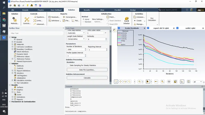
For each simulation, you need to show the convergence plot

Procedure-

1) Open Ansys workbench and drag Fluid Flow(Fluent) into project schematics , now double click on geometry to open space claim, here for CASE 1 open mixing tee short.SLDPRT

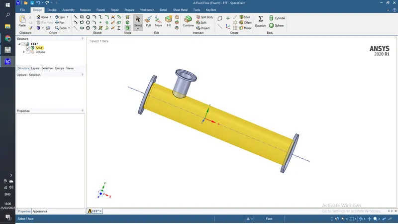
Now extract the fluid volume using Prepare>>Volume Extract

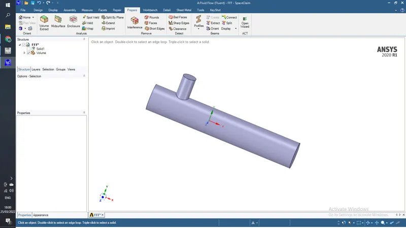
Now under strucutre tree right click on solid and click on suppress for physics. and exit space claim

Now double click on mesh module, here generate defualt mesh for the fluid.

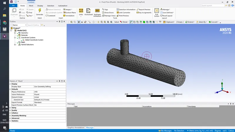
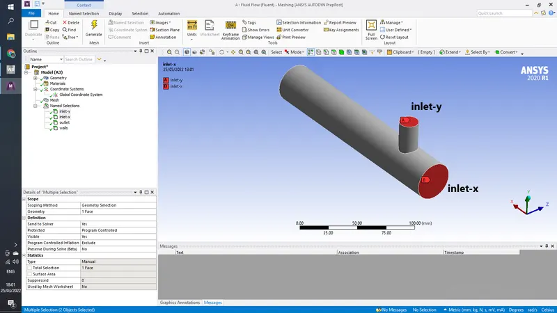
now using face selection, create named selection as follows

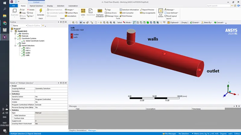
Now right click on mesh and click update to update the mesh in fluent

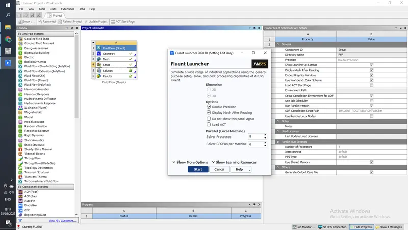
exit mesh and double click on Setup

here select the no. of core availiable and tick on double pricision

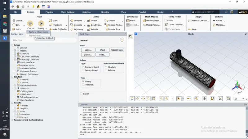
here perform a mesh check

let time be steady

solver type be pressure based

velocity formulation as absoulute

turn on energy

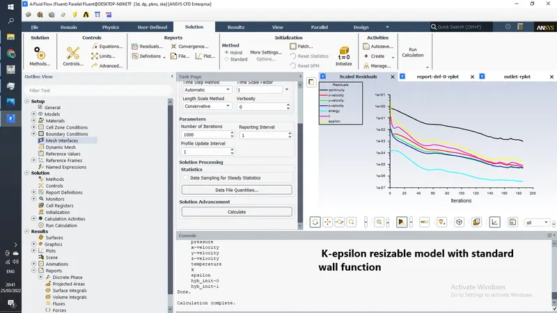
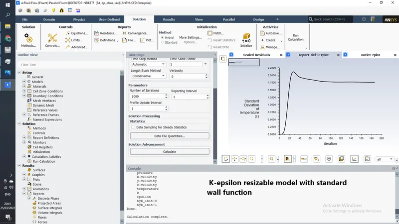
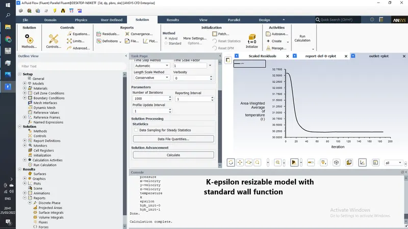
For CASE 1 Part 1, we will be using K-epsilon resizable model with standard wall function

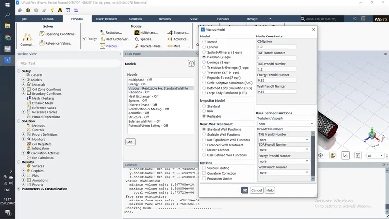
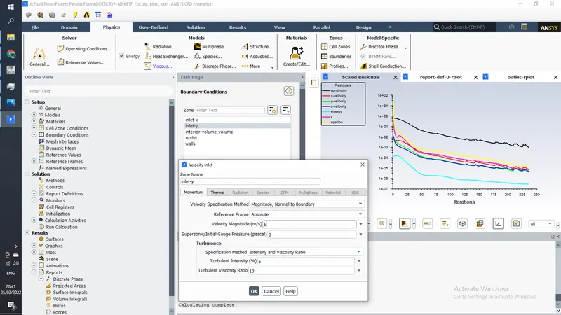
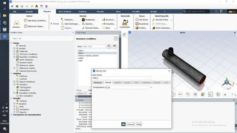
now go to boundaries and give inlet-y a velocity of 6 m/s and a tempraure of 19 degree celcius

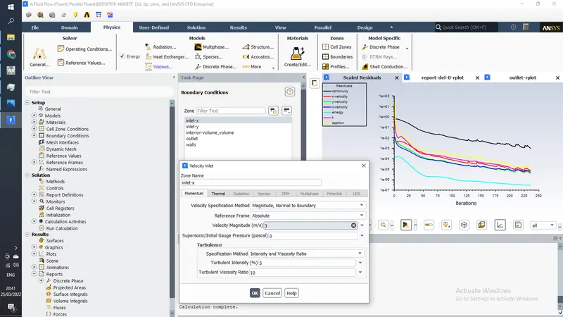
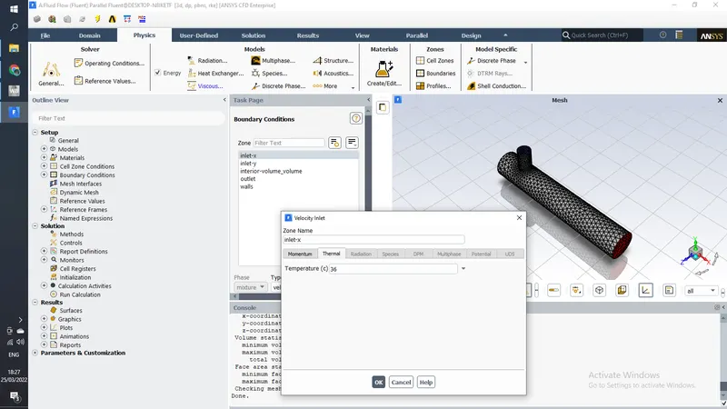
for inlet-x give velocity of 3 m/s and temprature as 36 degree celcius (momentum Ratio 2)

leave the rest boundry conditions be default

now go to solutions>>Definations>>new>>surface report>>area weighted average

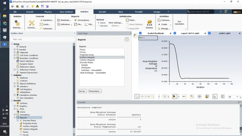
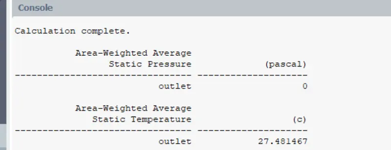
here create temprature report for the outlet

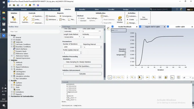
now add surface report>>standard deviation for outlet temprature also

now initialize the case using hybrid initalization

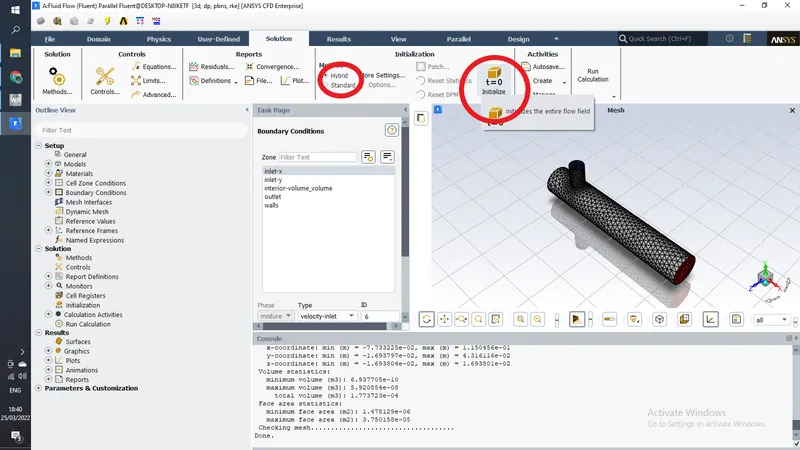
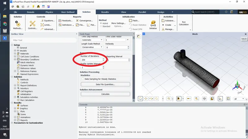
in calculations add 250 itrations

results

exit fluent and double click on results to open CFD Post

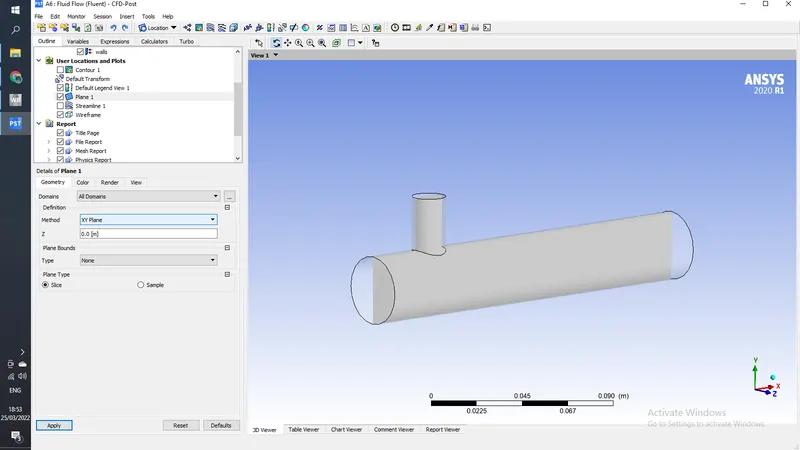
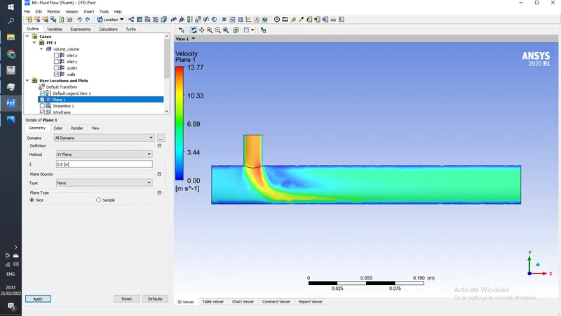
here add a plane in XY

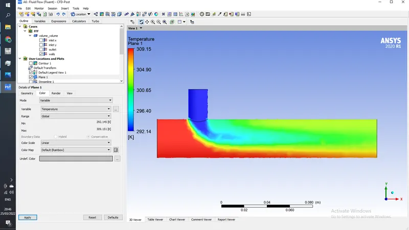
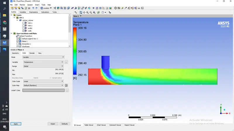
go to color>>mode>>variable>> temprature to see temprature along the plane

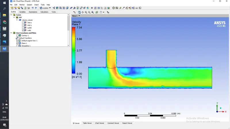
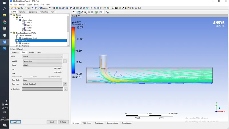
now change temprature to velocity

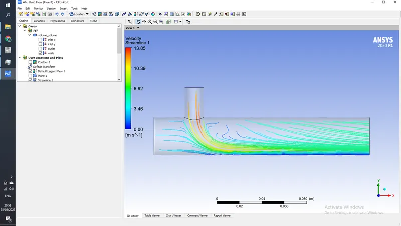
now add streamlines to show velocity lines across plane

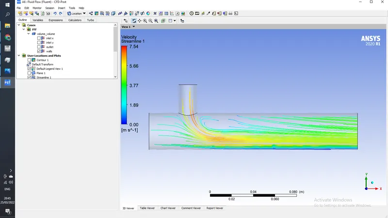
now exit cfd post and again open fluent

now use the k-omega SST model

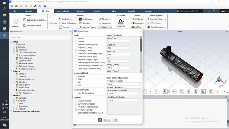
leave everthing rest same

therefore results are

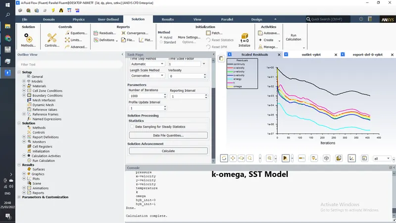
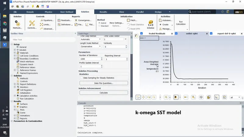
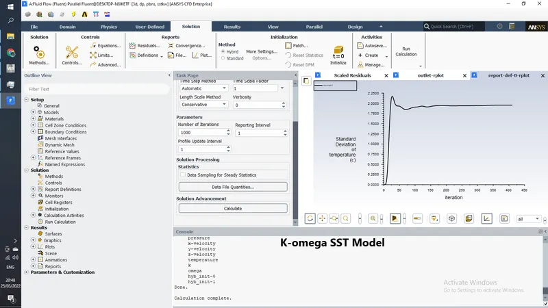
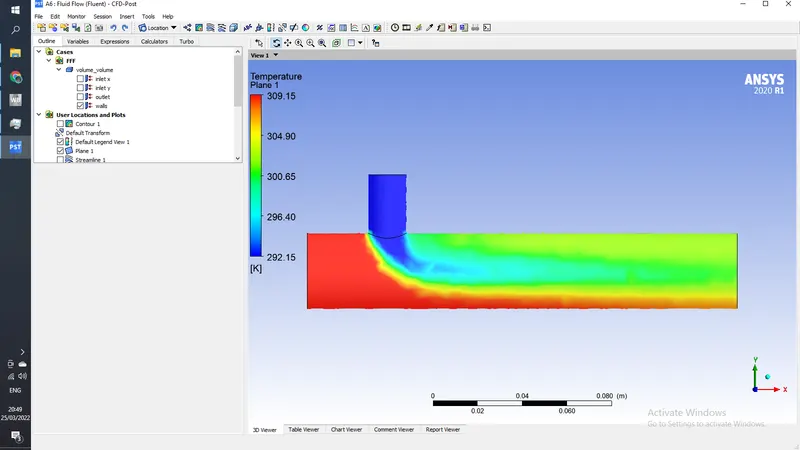
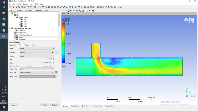
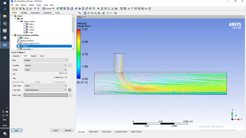
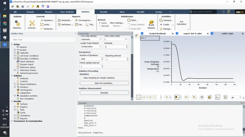
k-epsilon took less itration to converge as compared to k-omega

also the turbulance in ek-epsilon model is more as in the velocity contours the inlet-y velocity fades as it travels further in pipe as compared to one in k-omega, k-omega is also most commonly used, so we will be using k-omega model.

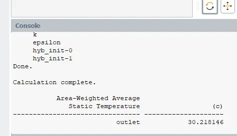
results from k-epsilon model

Analytical results

T(mix)= (m(hot)*T(hot) + m(cold)*T(cold))/m(hot)+m(cold)

here m= mass flow rate= p*A*V

p=1.225 kg/m3

T(hot)= temprature of hot inlets= 36 degree celcius

T(cold)= temprature of hot inlets= 19 degree celcius

T(mix) = mixed temprature at outlet

A(hot)= 0.9m2

A(cold)= 0.226m2

V(hot)= 3 m/s

V(cold)= 6 m/s

Therefore T(mix)= 30.03

now for moment ratio 4, we will be increasing the inlet-y speed to 12 m/s

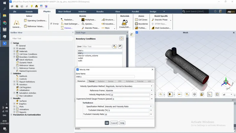
again initialize the model

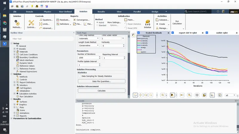
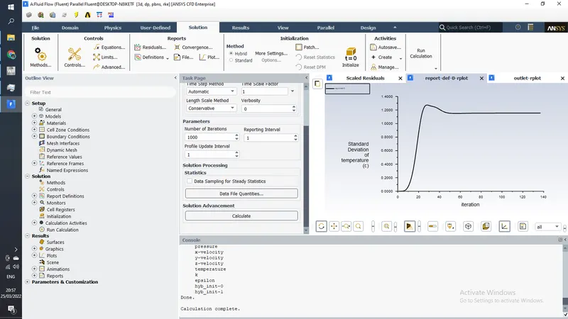
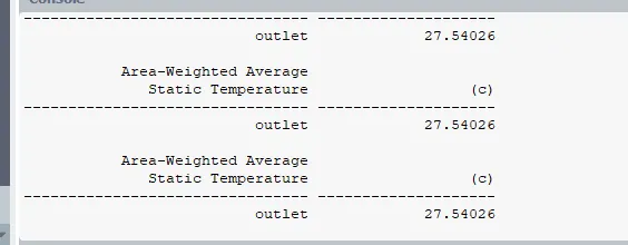
results

Analytical results

T(mix)= (m(hot)*T(hot) + m(cold)*T(cold))/m(hot)+m(cold)

here m= mass flow rate= p*A*V

p=1.225 kg/m3

T(hot)= temprature of hot inlets= 36 degree celcius

T(cold)= temprature of hot inlets= 19 degree celcius

T(mix) = mixed temprature at outlet

A(hot)= 0.9m2

A(cold)= 0.226m2

V(hot)= 3 m/s

V(cold)= 12 m/s

Therefore T(mix)= 27.71

CASE 2

The setup for this case will be same as the last case, including mesh size, model used etc, only velocity at inlets will be change according to requirments

Part 1

inlet-y - 6 m/s

inlet-x 3 m/s

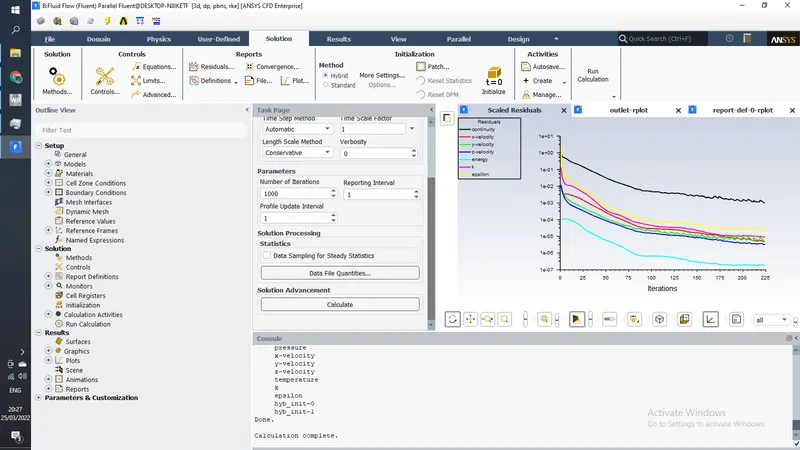
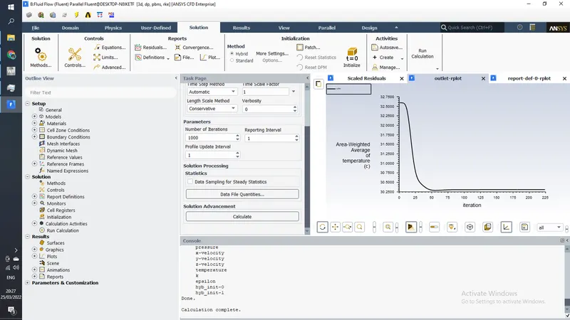
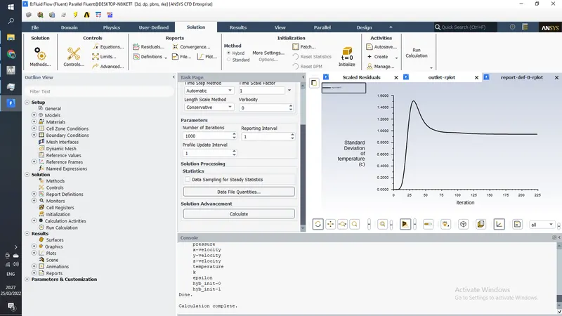
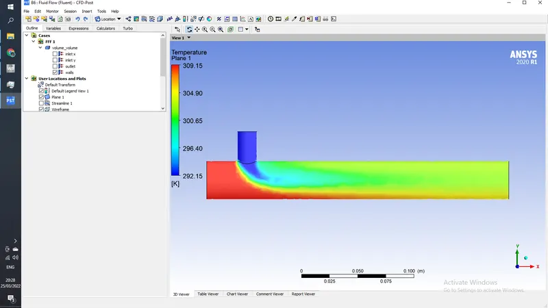
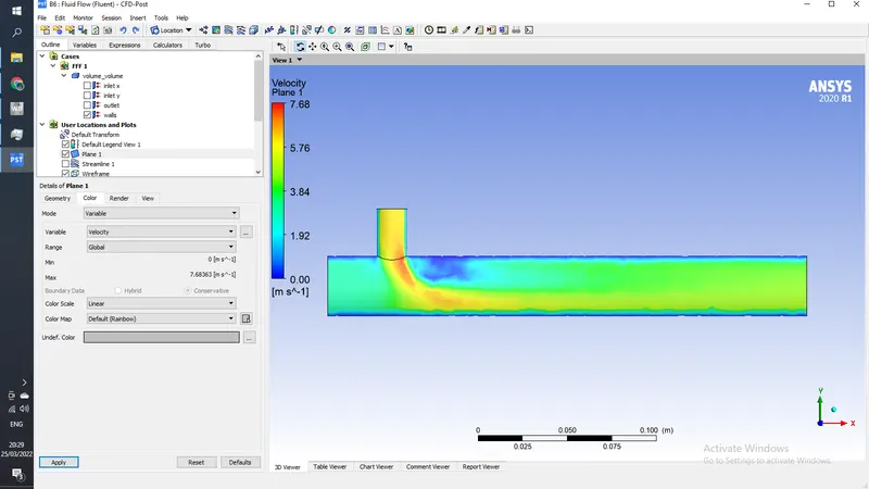
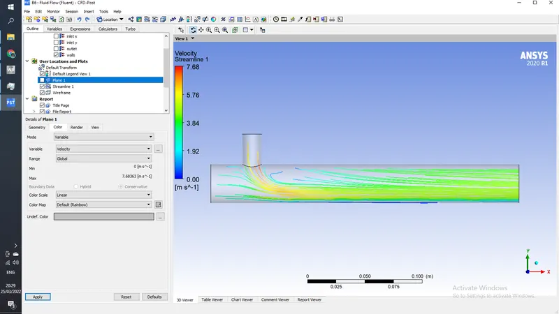
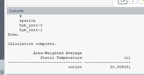
Analytical results

T(mix)= (m(hot)*T(hot) + m(cold)*T(cold))/m(hot)+m(cold)

here m= mass flow rate= p*A*V

p=1.225 kg/m3

T(hot)= temprature of hot inlets= 36 degree celcius

T(cold)= temprature of hot inlets= 19 degree celcius

T(mix) = mixed temprature at outlet

A(hot)= 0.9m2

A(cold)= 0.226m2

V(hot)= 3 m/s

V(cold)= 6 m/s

Therefore T(mix)= 30.03

now changing inlet-y velocity to 12 m/s

Analytical results

T(mix)= (m(hot)*T(hot) + m(cold)*T(cold))/m(hot)+m(cold)

here m= mass flow rate= p*A*V

p=1.225 kg/m3

T(hot)= temprature of hot inlets= 36 degree celcius

T(cold)= temprature of hot inlets= 19 degree celcius

T(mix) = mixed temprature at outlet

A(hot)= 0.9m2

A(cold)= 0.226m2

V(hot)= 3 m/s

V(cold)= 12 m/s

Therefore T(mix)= 27.71

Conclusion-

1) Analytical Calculation results and simulation results are very close to each other.

2) the increased momentum ratio resulted in less standard deviation then the one with less momentum ratio

3) increasing length dosen't give any significance in results, in both cases redults are almost same

4)

CASE	cell count	Average outlet temperature	Number of iterations for convergence
1	12728 elements	part 1-30.21 , part 2- 27.54	part 1-190 , part 2- 130
2	15483 elements	part 1- 30.30 , part 2- 27.48	part 1- 225 , part 2- 150