Week 1- Mixing Tee

AIM:

To perform steady-state turbulence model simulations in Ansys fluent solver, to compare the mixing effectiveness when hot inlet temperature is 36⁰C and the Cold inlet is at 19⁰C.

OBJECTIVES:

To perform turbulence modelling for two versions of mixing tee.

• Case(1) - Short mixing tee with a hot inlet velocity of 3m/s of momentum ratio of 2 and 4.
• Case(2) - Long mixing tee with a hot inlet velocity of 3m/s of momentum ratio of 2 and 4.

working fluid - air

Perform the turbulence simulation by using k-epsilon and k-omega SST models for case(1) and the model which predicts better results is used to model the case(2).

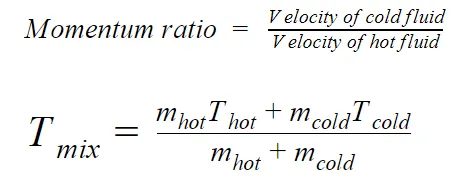
FORMULAE:

INTRODUCTION:

Mixing Tee geometries are primarily used as energy exchange devices, where fluids at different temperatures are mixed at T-Junction. Mixing Tee geometries are widely used in many home and industrial applications. In HVAC, the mixing tee geometries are used to mix chilled air with outside fresh air. In the field of nuclear reactor safety, since mixing leads to highly transient temperature fluctuations and cyclic thermal stresses at pipe walls results in thermal fatigue and thermal failure of pipeline.

In this report, mixing tee geometry of HVAC application is considered. Different parameters such as length of the geometry, velocity of inlet fluids and how these parameters affect the mixing efficiency are validated in this report.

Turbulence models -

In CFD, different approaches have been implemented to perform turbulence modeling.

(a) Reynolds-averaged Navier-Stokes simulation (RANS) - In this method, the Navier stokes equations are approximated by mean flow parameters and transport equations are used to perform turbulence modelling.

ModifiedNavier stokes momentum equation by using RANS based method

where,

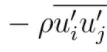is the extra term and is defined as Reynolds (or) Turbulence stress tensor.

The Reynolds stress tensor is approximated by using Boussinesq hypothesis as shown below.

, where μt is eddy viscosity.

Different models are introduced to calculate eddy viscosity. k-epsilon and k-omega are famously used RANS models to calculate eddy viscosity.

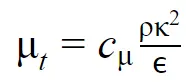
• K-epsilon model - K is turbulent kinetic energy extraction rate from mean flow, epsilon(ε) is rate of dissipation of turbulent kinetic energy. In this model, Transport equations for k and ε are used to calculate eddy viscosity. The limitations of k-ε model is, it is not accurate at predicting boundary layers with adverse pressure gradients

• K-omega model - K is turbulent kinetic energy extraction rate from mean flow, omega(ω) is rate of dissipation of turbulent kinetic energy. In this model, Transport equations for k and ω are used to calculate eddy viscosity. The limitations of k-ω model is, it is not suitable for free stream flow.

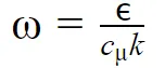
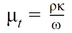
• K-ω SST model - In k-ω model, the wall shear stress is over predicted. So, k-ω SST model is introduced, where viscous limiters are used to control the over predicting of wall shear stress. This model gives better results for external aerodynamics simulations compared to k-ω model.

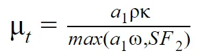
(b) Large eddy simulation (LES) - This method can visualize formulation of eddies and boundary layer seperation more accurately. In LES, subgrid scale model is used to viaualize smaller eddies. The turbulence kinetic energy is used to validate the model.

(c) Direct numerical simulation (DNS) - In this method, the Navier-Stokes equations are solved to obtain the solutions. This is the best accurate method, but the limitation of this method is the computational time to solve the model is very high. Even super computers take a huge amount of time to solve the models by this method.

ACCUARACY OF TURBULENCE MODELS - DNS > LES > RANS

COMPUTATIONAL TIME - DNS > LES > RANS.

NOTE - In engineering applications, RANS model is widely used.

PROCEDURE:

ANSYS FLUENT software is used for turbulence modelling.

CASE 1(a) - SHORT MIXING TEE _ momentum ratio - 4

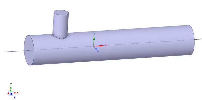
Geometry dimensions - Diameter of cylinder (Length along x-axis) = 0.0339 m

Diameter of cylinder (Length along y-axis) = 0.017 m

Length of cylinder (x-axis) = 0.1924 m

Meshing -

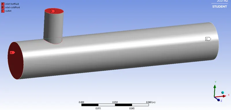
The boundaries are defined by using named selections as shown in the fig.

Hot fluid enters at secton A, Cold fluid enters at section B, Mixed fluid leaves at section C.

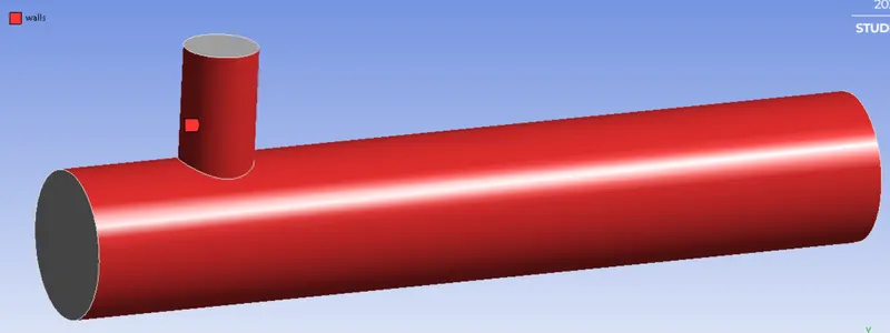
Next, mesh the geometry. Since, the geometry is a solid model, tetrahedron elements are formed.

Element size	1.02e-2 m
No.of elements	12,444

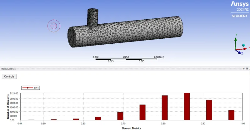
Generally, it is prefereed to have element quality > 5%. In this model, since the minimum element quality is greater than 44%, it is considered for analysis.

After meshing is done, the numerical simuation is done by giving inputs in the setup model.

Setup -

(a) k - ε model :

Before setting up the model, the mesh check is performed to check the generated mesh obeys the minimum qulaity criteria. The dimensions of minimum and maximum element can be checked.

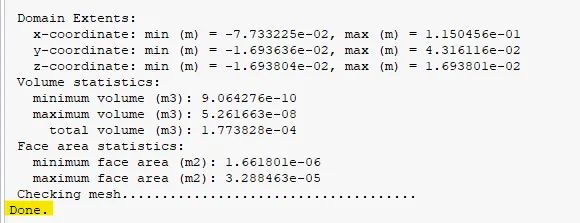
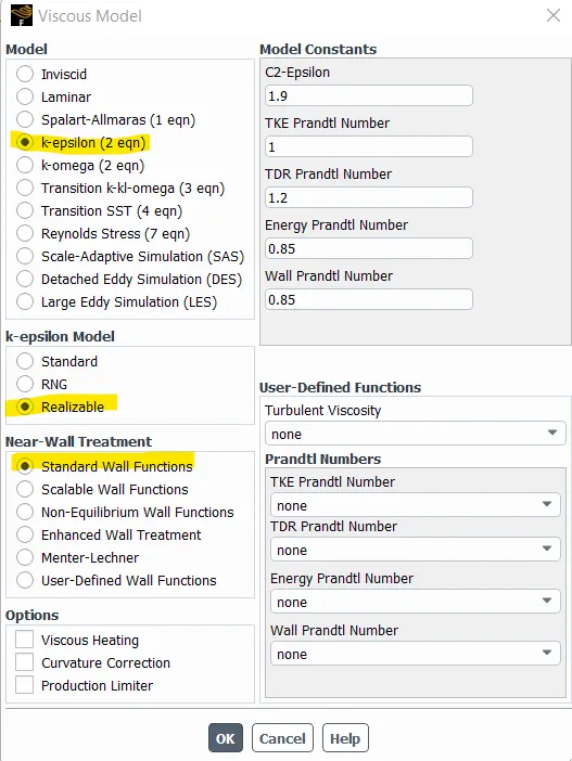
Setting up physics : Solver

Time - Steady state

Type - Pressure based

Velocity formulation - Absolute type

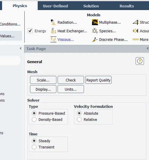
Turbulence model - k - ε model

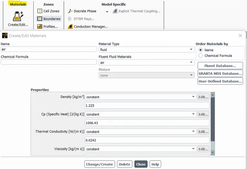
Working fluid - air

Boundary conditions -

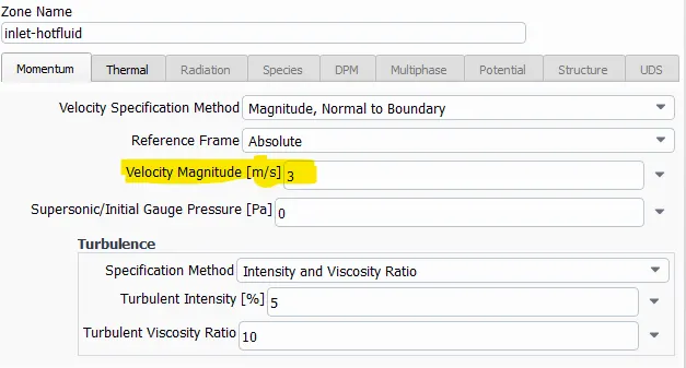
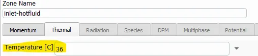
Inlet hot fluid -

Type - velocity inlet, velocity magnitude = 3m/s, Temperature = 36 degree celsius.

Inlet cold fluid -

Type - velocity inlet, velocity magnitude = 12m/s, Temperature = 19 degree celsius.

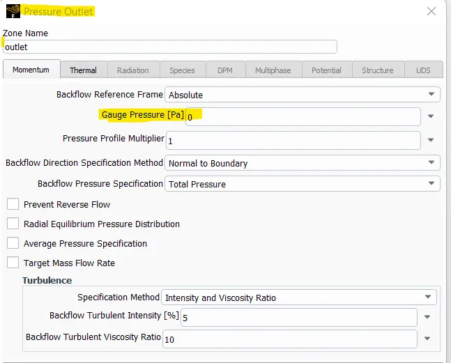
Outlet -

Type - Pressure outlet, Gauge pressure = 0 Pa

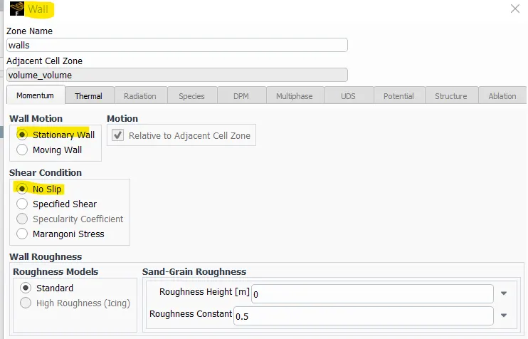
Walls -

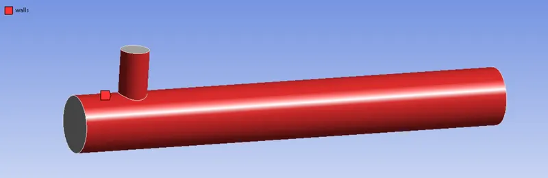
Type - wall, no slip boundary conditions are applied.

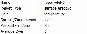
Reports -

To monitor the physical quantities, reports are generated, so that physical variables at each iteration is plotted.

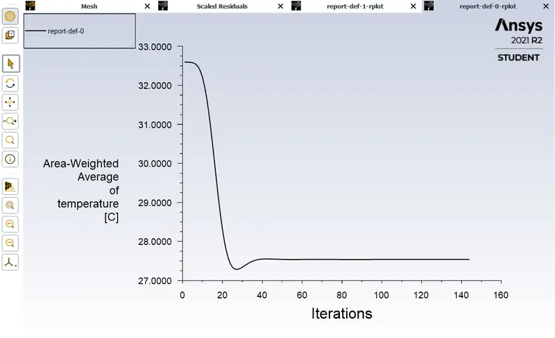
1) Outlet temperature - In order to predict the effecectiveness of mixing tee geometry, outlet temp is considered.

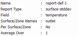
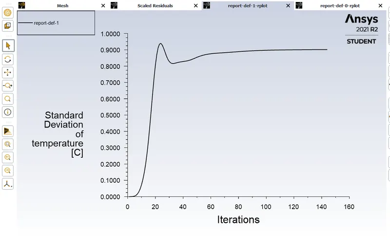
2) Outlet temperature standard deviation - In order to predict the effectiveness of mixing, the standard deviation of outlet temperature is compared. Lower the standard deviation indicates good mixing of fluids.

Simulation -

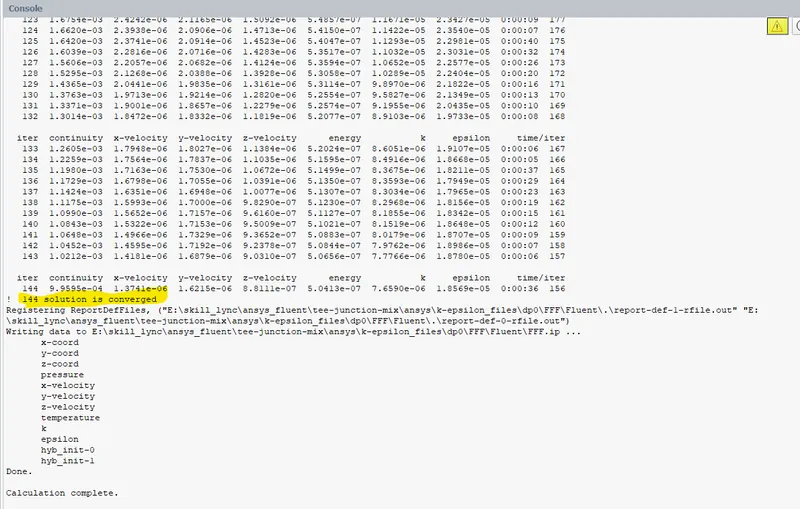
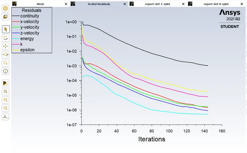
The solution is converged at 144 iteration.

(b) k-ω model :

For simulation of k-ω sst turbulence model, select k-omega(2 eqn) in physics model as shown in the fig.

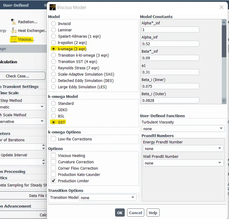
The boundary conditions are same as k-ε model.

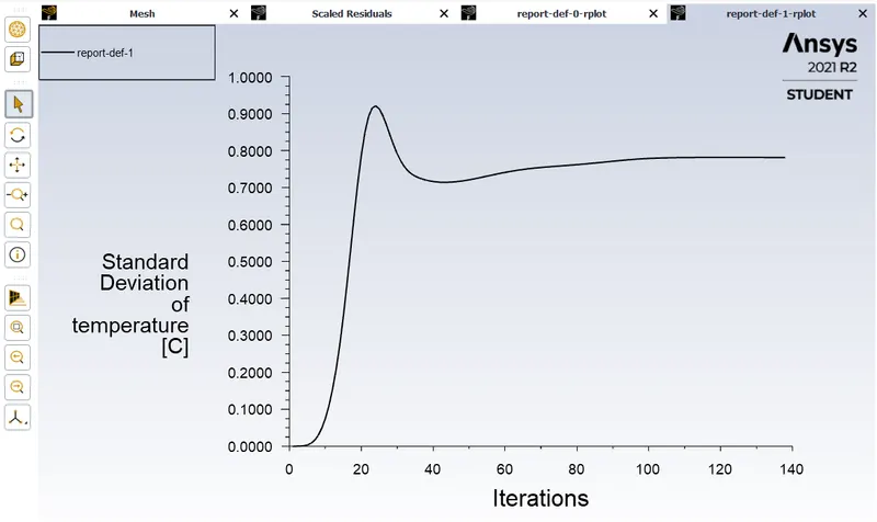
Simulation -

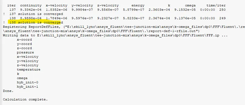
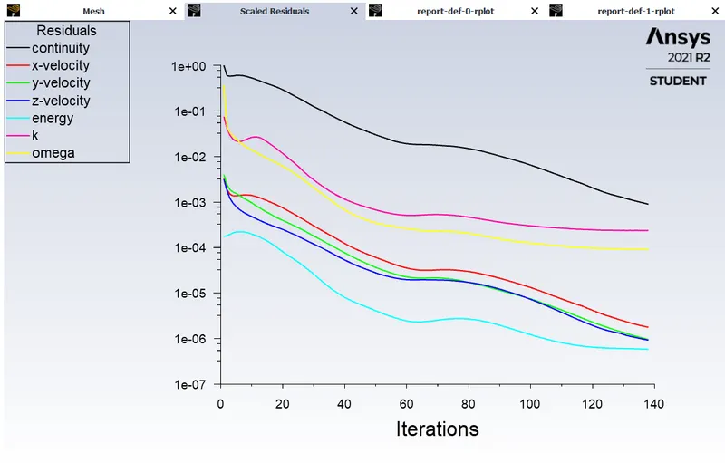
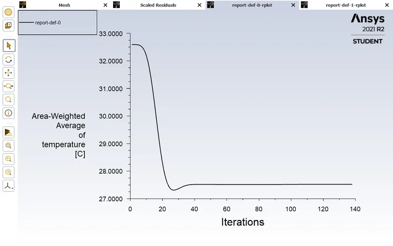
The solution is converged at 138 iteration step.

Analytical solution -

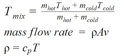
From the above equations, Tmix = ((0.0009*3)(36^2) + (0.0002*12)(19^2)) / (0.0009*3*36 + 0.0002*12*19)

Tmix = 30.57 degree celsius

Comparision of k-ε and k-ω SST model -

	k-ε model	k-ω SSTmodel
Total no.of iterations to converge	144	138
Average outlet temperature	27.53 degree celsius	27.52 degree celsius
Outlet temperature - standard deviation	0.90 degree celsius	0.78 degree celsius

From the tabel, the average outlet temperature in both the models are nearly same, but of absolute percentage error 9.94%. The standard deviation of outlet temperature in k-ω SST model is lesser than k-ε model, more uniform temperature is obtained in k-ω SST model. The convergence rate in k-ω SST model is greater than k-ε model. So, by considering the above results, it is estimated that k-ω SST model gives accurate results.

So, k-ω SST model is used to model remaining cases.

CASE 1(b) - SHORT MIXING TEE _ momentum ratio - 2

In this case, Since momentum ratio is 2, cold fluid inlet velocity is 6m/s.

The remaining steps and process is same as case 1(a) model.

Analytical solution -

From the above equations, Tmix = ((0.0009*3)(36^2) + (0.0002*6)(19^2)) / (0.0009*3*36 + 0.0002*6*19)

Tmix = 32.77 degree celsius

Simulation -

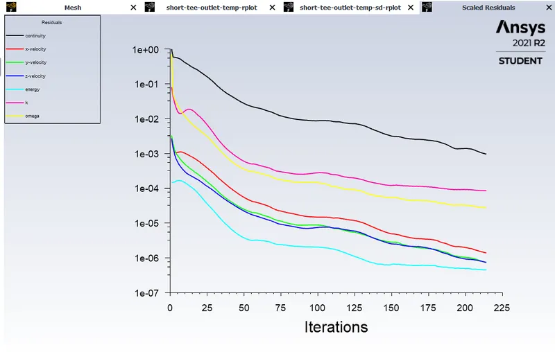
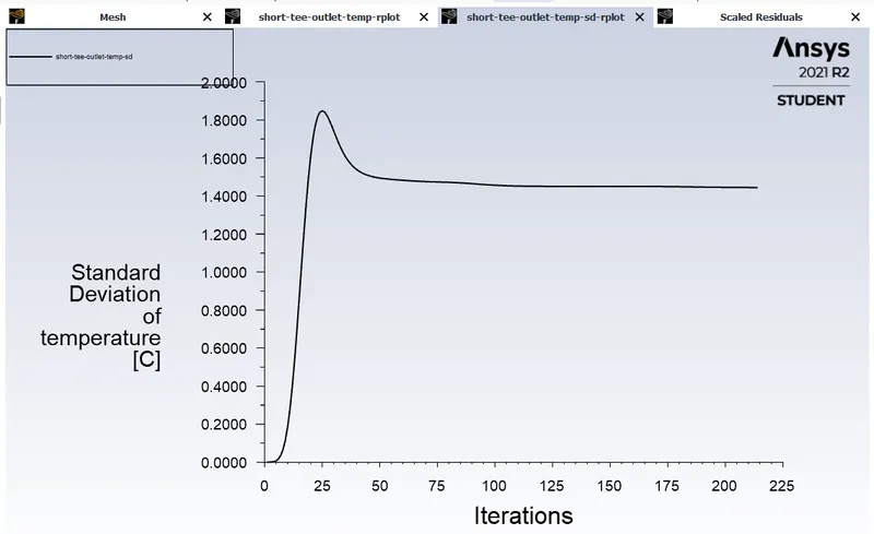
The solution is converged at 214 iteration step

Residual plot

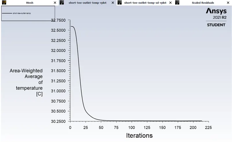
Average outlet temperature is 30.26 degree celsius. The absolute percentage error with analytical solution is 7.65%

Standard deviation of outlet temperature is 1.44 degree celsius

CASE 2(a) - LONG MIXING TEE _ momentum ratio - 2

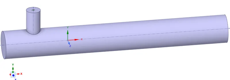
Geometry dimensions - Diameter of cylinder (Length along x-axis) = 0.0339 m

Diameter of cylinder (Length along y-axis) = 0.017 m

Length of cylinder (x-axis) = 0.2678 m

Meshing -

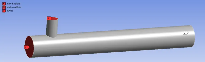
The boundaries are defined by using named selections as shown in the fig.

Hot fluid enters at secton A, Cold fluid enters at section B, Mixed fluid leaves at section C.

Next, mesh the geometry. Since, the geometry is a solid model, tetrahedral elements are formed.

Element size	1.38e-2 m
No.of elements	15,562

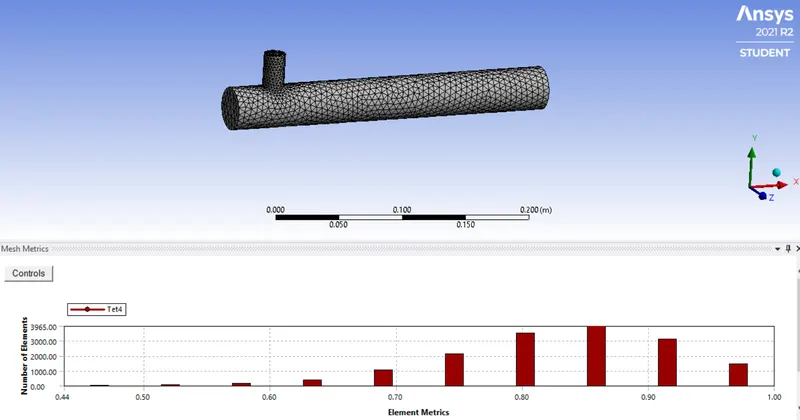
Generally, it is prefereed to have element quality > 5%. In this model, since the minimum element quality is greater than 44%, it is considered for analysis.

After meshing is done, the numerical simuation is done by giving inputs in the setup model.

Setup -

k-ω SST model is used to perform the simulation.

The setup conditions are given similar to short tee mixing model.

Simulation -

The solution is converged at 267 iteration step.

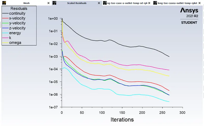
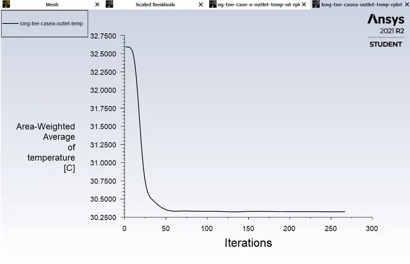
Average outlet temperature is 30.32 degree celsius. The absolute percentage error with analytical solution is 7.47%

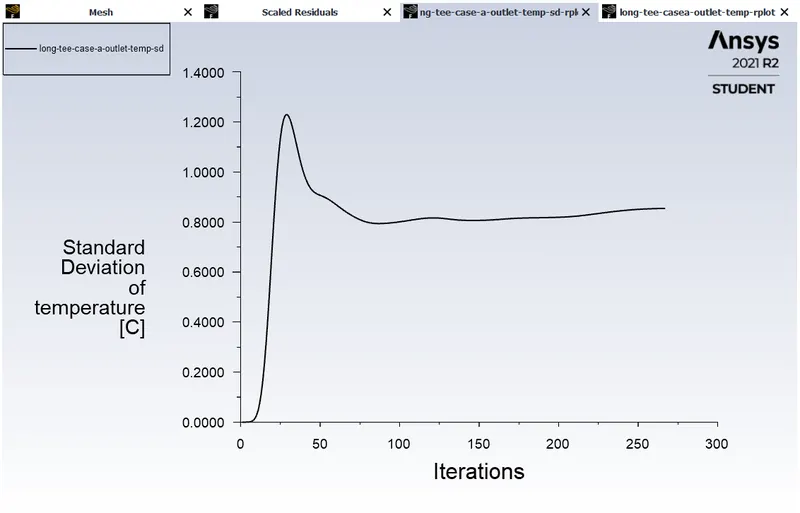
Standard deviation of outlet temperature is 0.85 degree celsius

CASE 2(b) - LONG MIXING TEE _ momentum ratio - 4

Simulation -

The solution is converged at 329 iteration step.

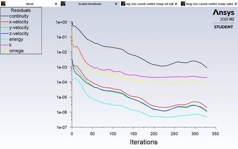
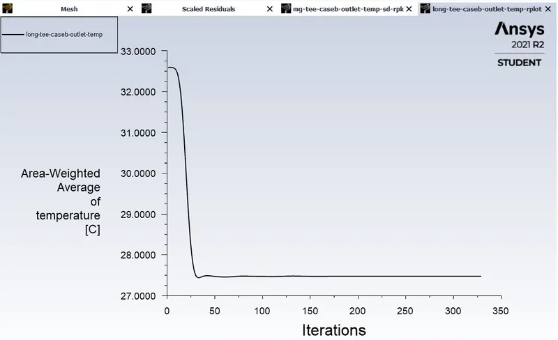
Average outlet temperature is 27.47 degree celsius. The absolute percentage error with analytical solution is 10.11%

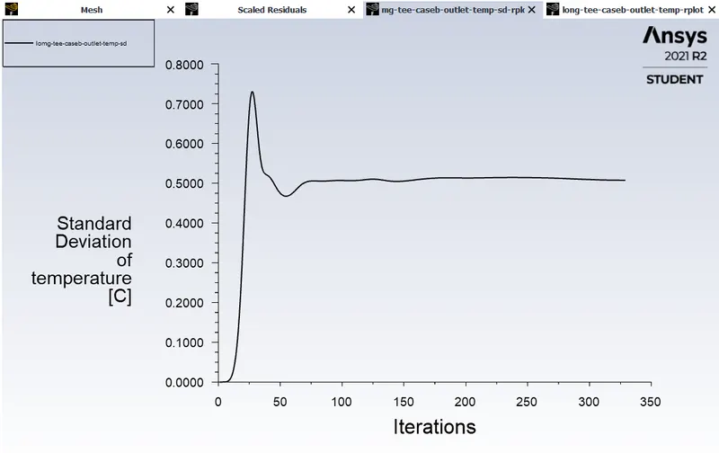
Standard deviation of outlet temperature is 0.5 degree celsius

RESULTS -

Contour plots of Short mixing tee of momentum ratio 2 and 4.

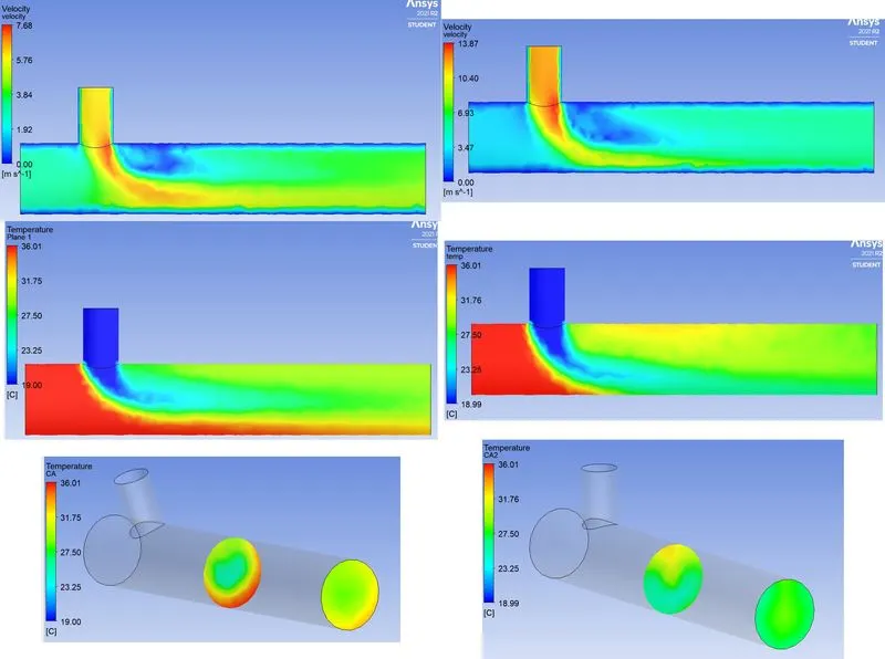
Contour plots of long mixing tee of momentum ratio 2 and 4.

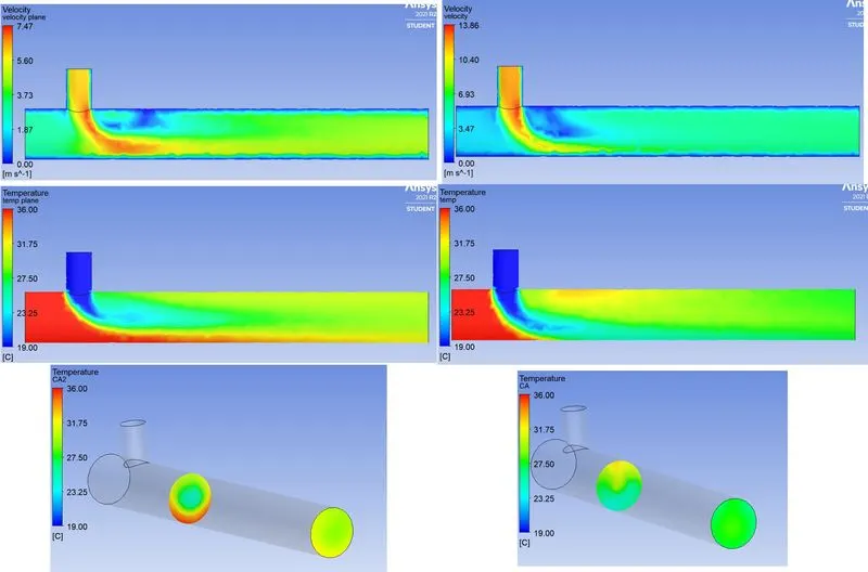
From the above fig, it is observed that

• From velocity contours, the blue region near the walls indicates the boundary layer separation region.
• From temperature contours, in both short and long mixing tee geometries, as the momentum ratio increases, more uniform temperature is obtained at the outlet.

S.No	Model	Analytical temperature after mixing	Outlet Temperature	Standard deviation of temperature at outlet	Iterations to converge
1	Short mixing tee (momentum ratio = 2)	32.77 degree celsius	30.26 degree celsius	1.44 degree celsius	214
2	Short mixing tee (momentum ratio = 4)	30.57 degree celsius	27.52 degree celsius	0.78 degree celsius	137
3	Long mixing tee (momentum ratio = 2)	32.77 degree celsius	30.32 degree celsius	0.85 degree celsius	267
4	Long mixing tee (momentum ratio = 4)	30.57 degree celsius	27.49 degree celsius	0.5 degree celsius	329

From the table, it is observed that

• As length of mixing tee increases, of same initial conditions, average outlet temperature is almost same but the standard deviation of outlet temperature is decreased, which indicates more uniform temperature is obtained.
• As momentum ratio increased from 2 to 4, of same mixing tee length, more uniform temperature is obtained at outlet.
• So, the effectiveness of mixing tee increases when the momentum ratio, length of the geometry is increased.

Grid Independency -

The analytical temperature for momentum ratio 4 is 30.57 degree celsius.

S.No	Element size	No.of elements	Average outlet temperature	Standard deviation of outlet temperature	No.of iterations
1	0.0102 m	12,444	27.52 degree celsius	0.78 degree celsius	137
2	0.005 m	14,166	27.53 degree celsius	1.14 degree celsius	139
3	0.002 m	1,05,058	27.55 degree celsius	1.26 degree celsius	149

Table: Short mixing tee of momentum ratio 4

From the table, mesh gets finer as element size decreased from 0.01m to 0.002m, the no.of elements increases by a ratio of 8.4 but absolute percentage error is decreased from 9.97% to 9.87 %. Since accuracy is increased only by 0.1%, it is preferred to have a grid size of 0.0102m for short mixing tee.

S.No	Element size	No.of elements	Average outlet temperature	Standard deviation of outlet temperature	No.of iterations
1	0.0138 m	15,562	27.47 degree celsius	0.5 degree celsius	329
2	0.005 m	17,695	27.48 degree celsius	0.55 degree celsius	124
3	0.002 m	1,39,219	27.58 degree celsius	1.42 degree celsius	250

Table: Long mixing tee of momentum ratio 4

From the table, mesh gets finer as element size decreased from 0.0138m to 0.002m, the no.of elements increases by a ratio of 8.94 but absolute percentage error is decreased from 10.14% to 9.78%. Since accuracy is increased only by 0.36%, it is preferred to have a grid size of 0.0138m for a long mixing tee.

Flow chart of all cases in Ansys workbench -

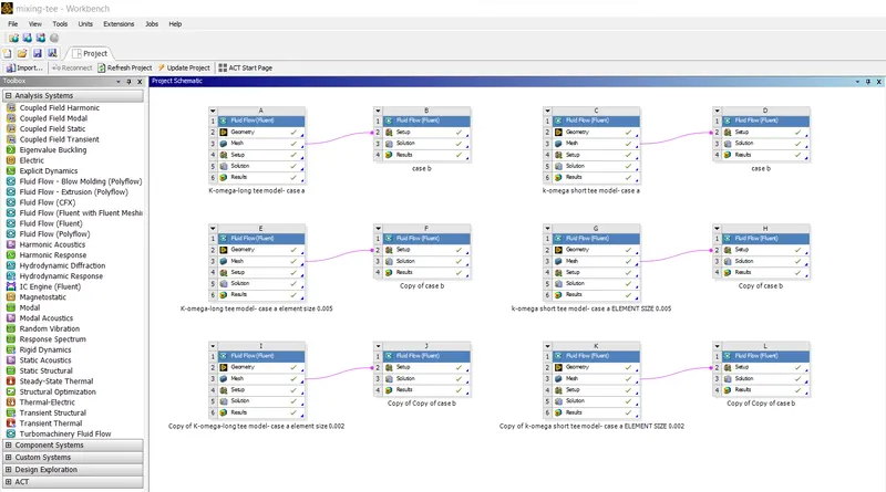
Conclusion:

It is concluded that, the effectiveness of mixing tee is improved for higher mixing length and higher momentum ratio from 2 to 4. Mesh independency for short mixing tee, long mixing tee is achieved for element size 0.012m , 0.0138m respectively.