Week 1- Mixing Tee

Aim of the project

• Steady state simulation of flow throught mixing Tee,
• compare the mixing effectiveness of the mixing Tee analytically and numerically when inlet temperatures are given,
• Use k-Epsilon and k- Omega models to get the proper judgement and then select the one for the next case.
• Simluate both the cases with two momentum ratios, compare the two cases for no. of cells, average outlet temperature, the number of iterations need for convergence

Problem set up

case (1) momentum ratio: 2

Simulation (a)

T_in_hot = 36 C, T_in_cold = 19C, v_in_hot = 3 m/s, v_in_cold = 6 m/s

We have to load the given geometry into the spaceclaim and extract the fluid volume from it, suppressing the actual model(supperess for physics) as we do not involve any wall into simulation as no heat transfer is there from wall to fluid.

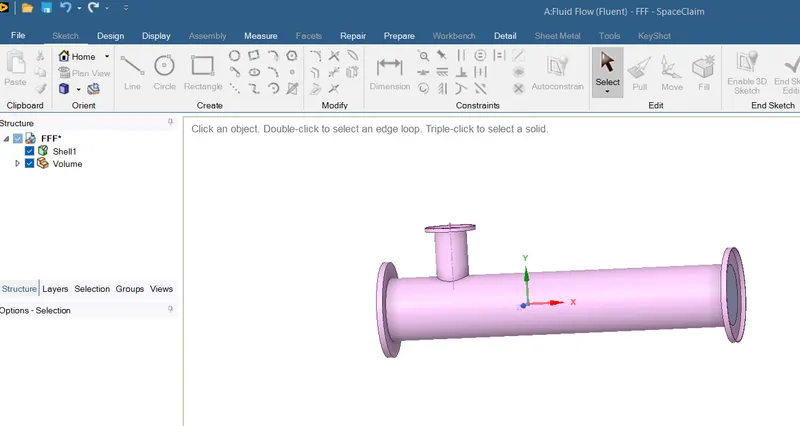
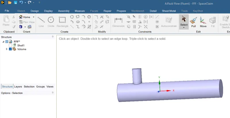
Now close the space claim. Now we go to meshing of the fluid section. We create named selection here as inlet_x, inlet_y, walls, outlet.

We can check meshing by cutting the fluid domain into a section as shown below to observe mesh flow. Then we investigate the mesh quality by clicking option element quality in quality section of mesh panel.

Now double click on set up option in Fluent cell for k-epsilon and k-omega methods.

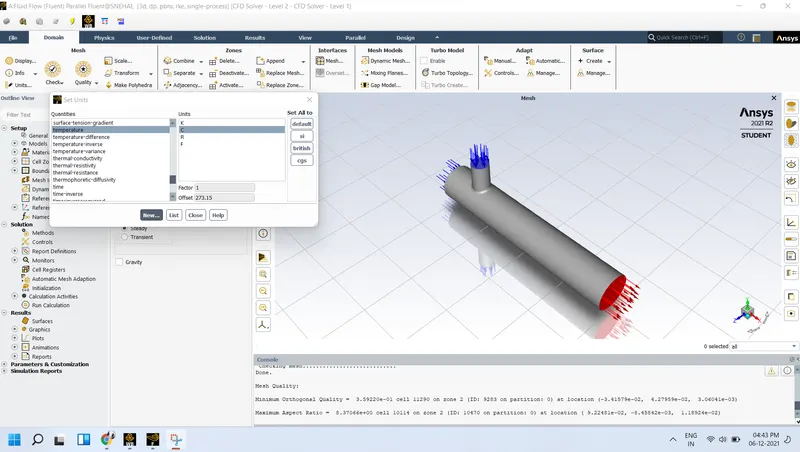
Then we are into Setup of FLUENT and we change unit of temperature from K to C.

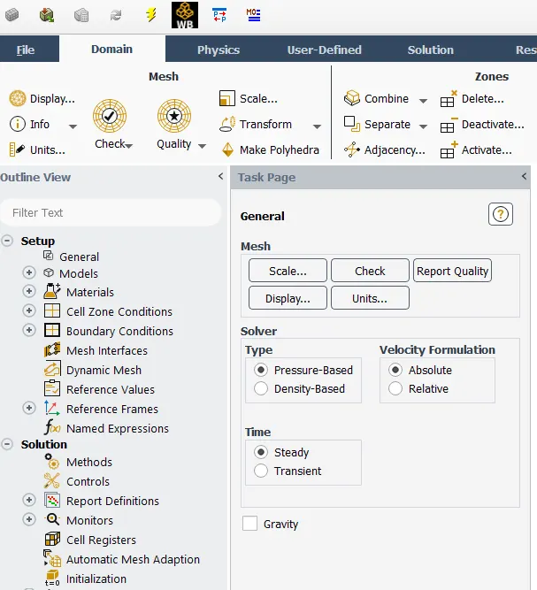
Now in general, we set solver: Pressure based solver, Velocity: Absolute and Time: Steady

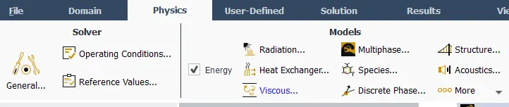
Next is as we want to to solve temperature dependent problem, we will enable energy equation.

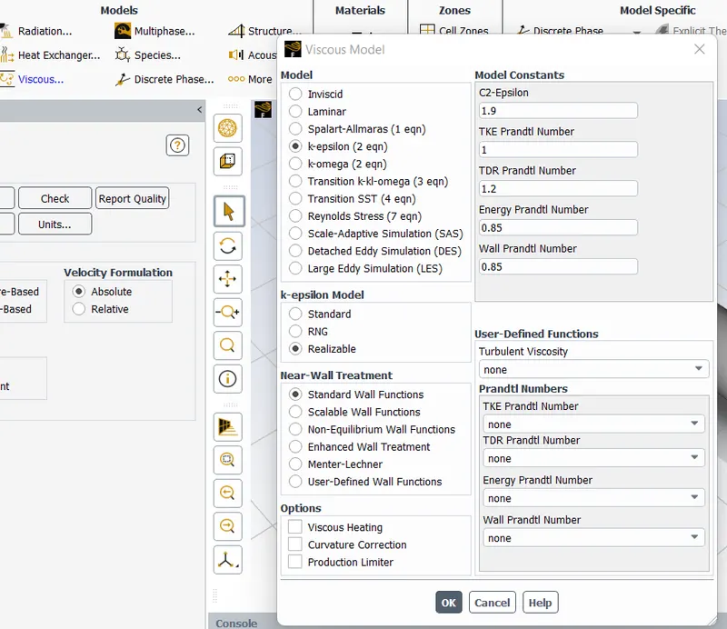
In viscous model, select 'k-Epsilon' Realizable for first simulation.

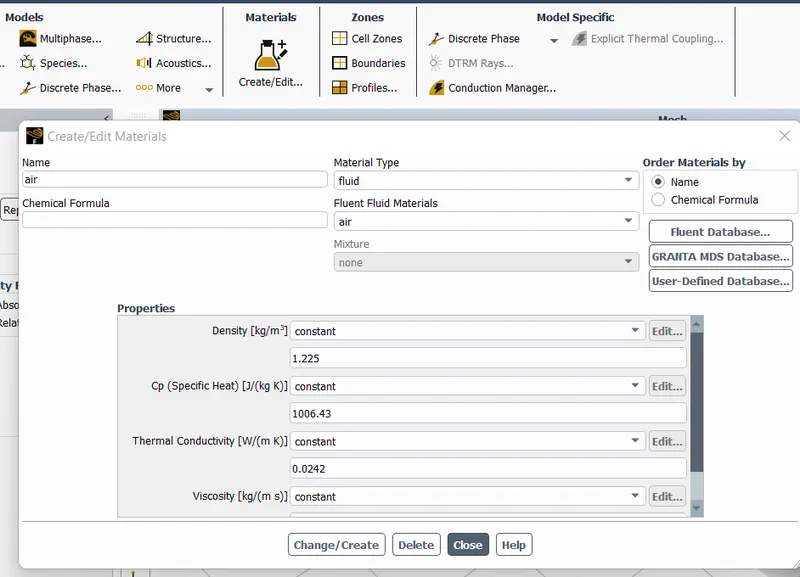
Now, in materials, click 'FLUENT database' to add new material if any. In present case, its air so keep it the default material.

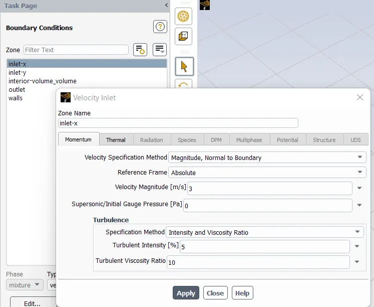
Now, let us set the boundary conditions as below,

inlet_x : in themral put temperature as 36 C and velocity as 3 m/s.

inlet_y : in thermal,put temperature as 19 C and velocity as 6 m/s.

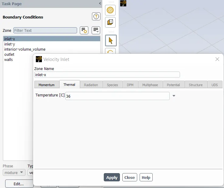
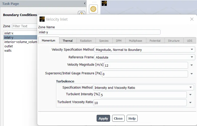
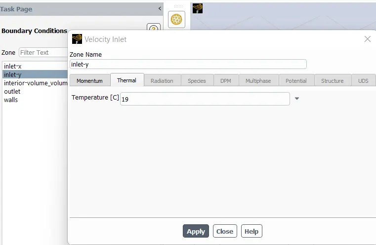
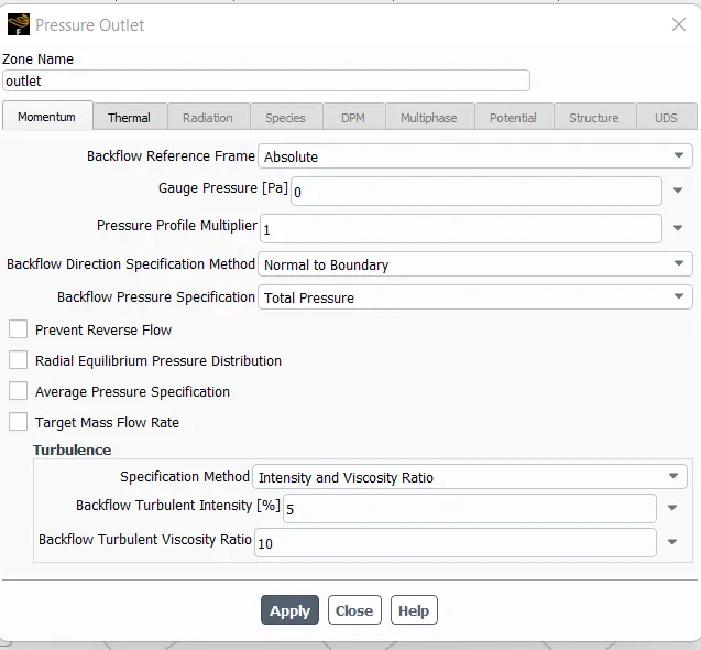
Now, set outlet pressure condition as atmospheric pressure value whihc is zero gauge pressure.

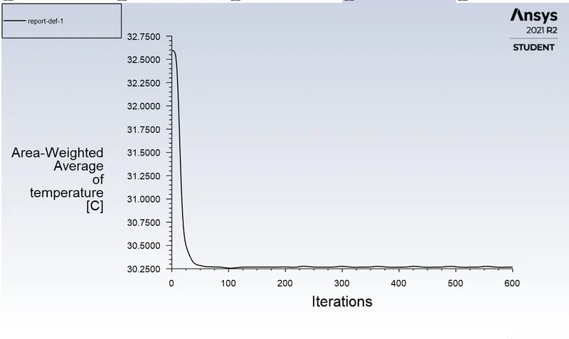
Now, in solution , reports, definitions, new, surface report monitor . Select area-weighted average.

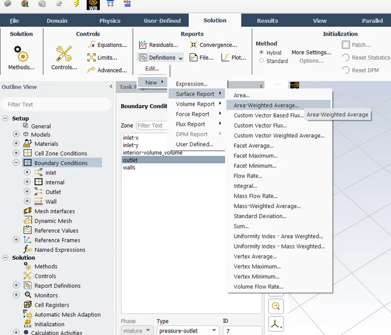
Here we want temperature average at outlet so select properly.

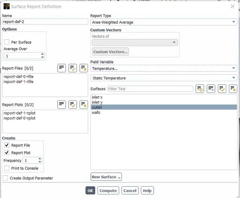
In similar way, create a plot for velocity plot at outlet boundary condition.

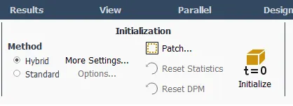
Now, we have to initialize the problem set up before running the simulation.

Initialization creates the initial solution that the solver will improve in coming iteartions. Standard initialization imposes the same values in all cells (We have to provide). We can improve this by patching different values into different zones like inlet/outlet. Patching and post-processing is not available after initiazation.

Hybrid initialization solves the Euler problem and it uses boundary conditions for solving. The solution to this equation is used as the initial guess.

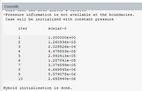
After clicking initializaion button, the below data is printed, basically it solves 10 equations and puts that initial guess value.

After this, we have to give no. of iterations and then press ' calculate'.

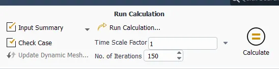
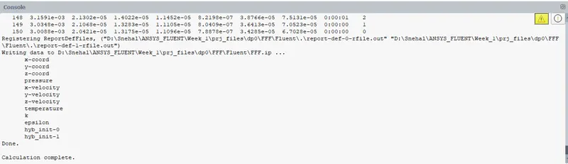
Next, below window will be seen so it means that calculation is complete.

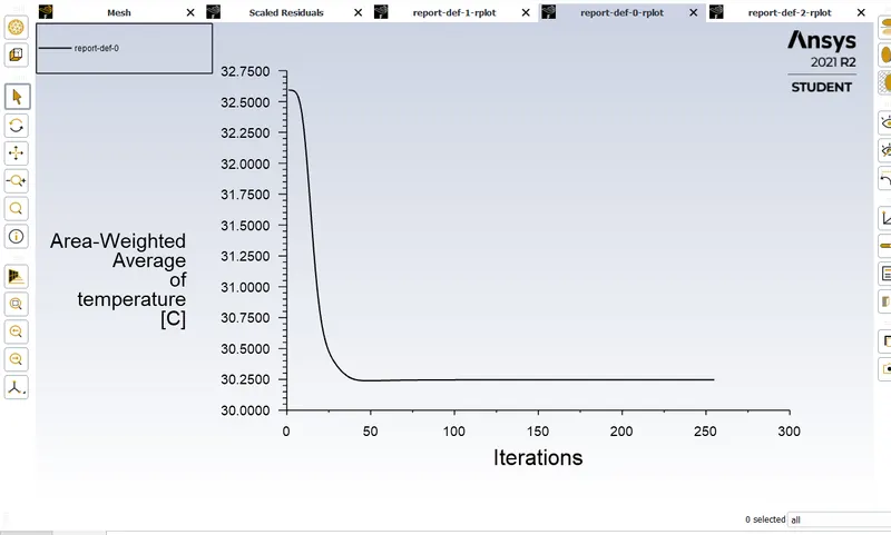
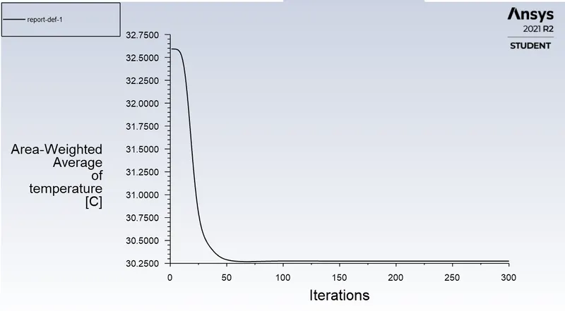
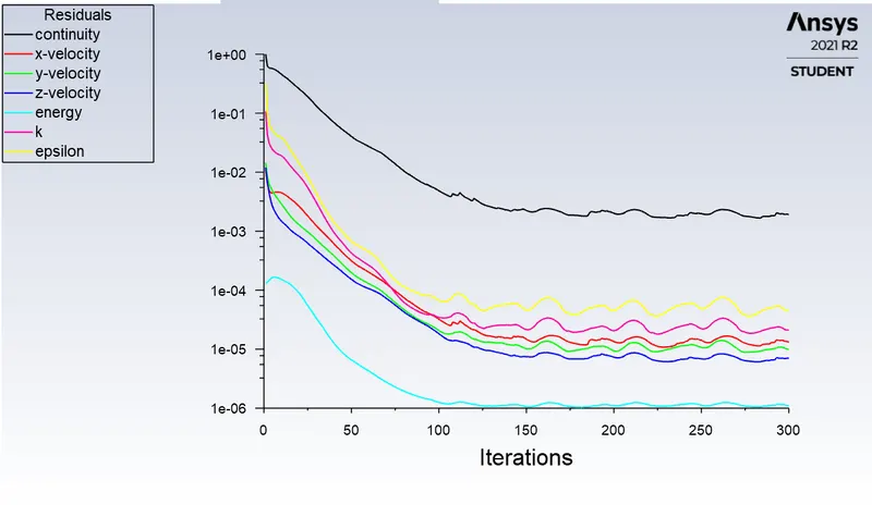
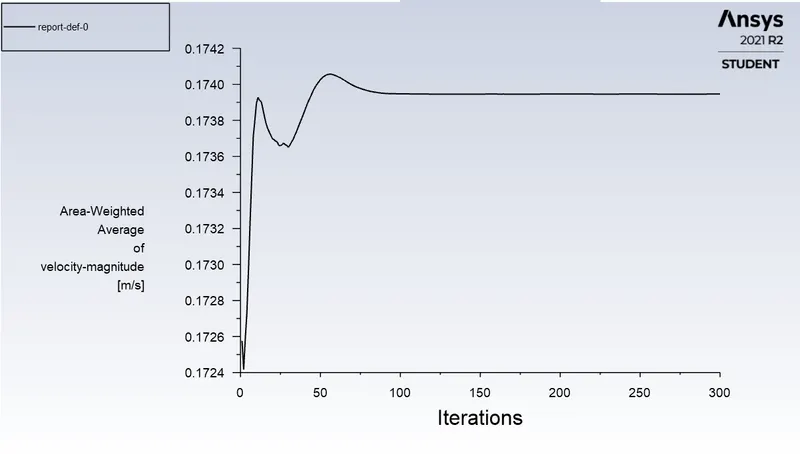
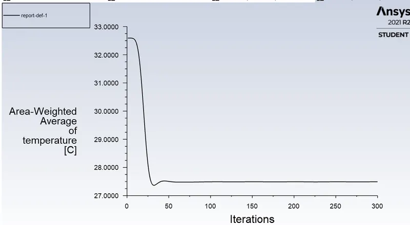
Below are the convergence plots for k-Epsilon method, also reports of temperatire and velocity at outlet.

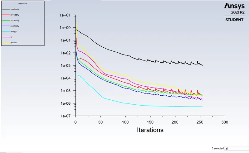
And residuals chart for energy equation will be below,

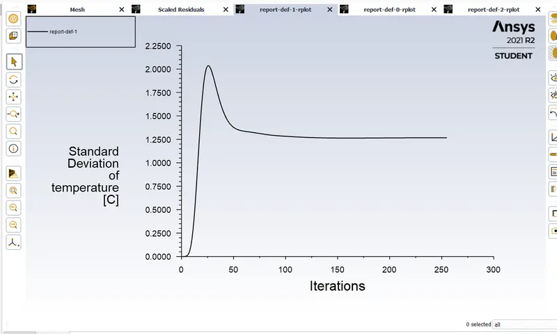
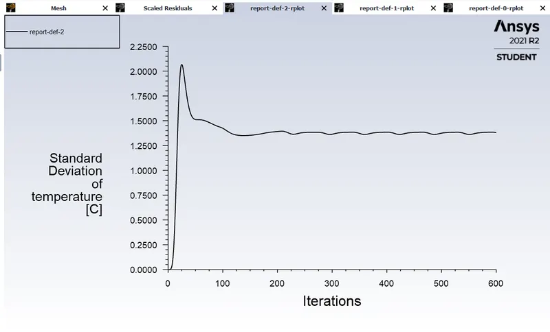
Standard deviation ,

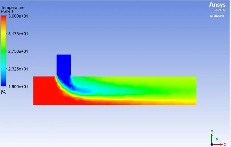
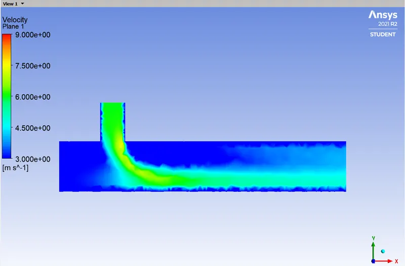
After this, we close the Fluent and start postprocessing. Now let us create a plane in xy direction and plot temperature and velocity profile on it. From the location menu, select plane , method 'XY' plane. Then accept X as 0. Press apply.

Then, select plane-1 (along pipe) from outline and in color, select variable, color by temperature, global and the contour will be generated as below,

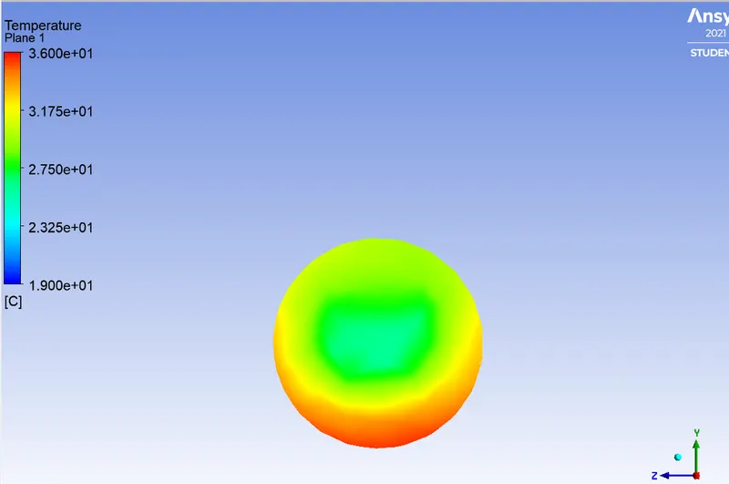
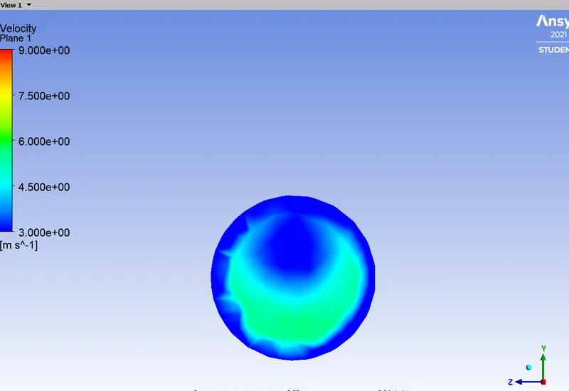
Now we create a plane in YZ direction to see the contours across the pipe and plot the contours,

Now, the same procedure is to be used for the k-Omega model .

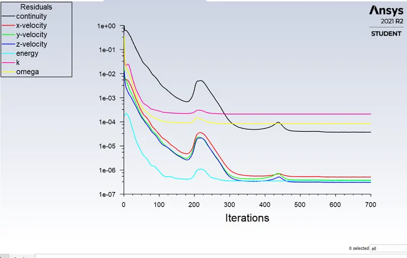
Below are the convergence plots for k-omega method, also reports of temperatire and velocity at outlet.

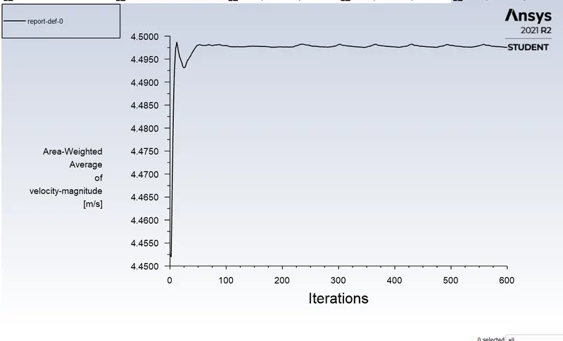
Now, in post-processing , we get below charts along and across the pipe,

Along pipe

a) Velocity contour

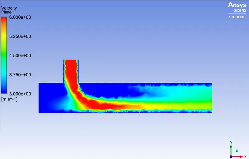
b) Temperature contour

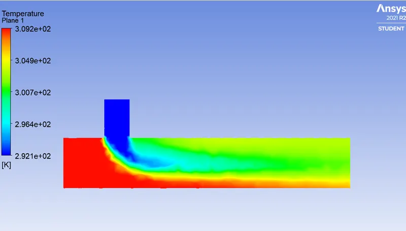
Across pipe

a) Velocity contour

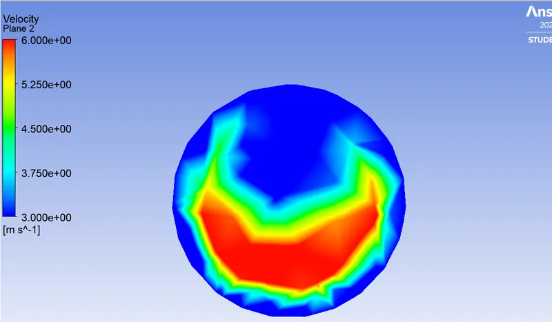
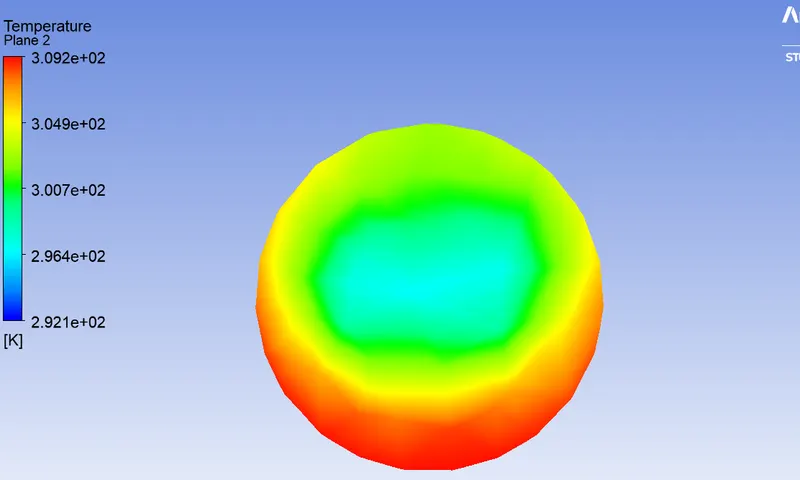
b) Temperature contour

Comparison table

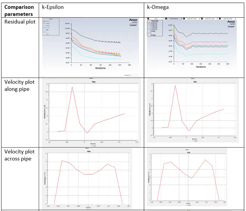
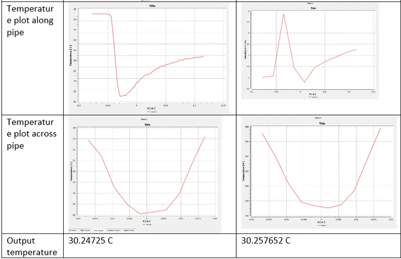
What model will be chosen for the goven situation of flow and why ?

k-Epsilon model is two equation model that gives a description of turbulence by means of two transport PDEs. The first transported variable is turbulent Kinetic energy, second is rate of dissipation of turbulent kinetic energy.

While, k-omega SST turbulent model is a two equation eddy-vsicosity model that is used in aerospace applications. It is mixed type model in which there is Wilcox k-omega and k-epsilon model. A blending function F1, activates the Wilcox model near wall and k-epsilon in free stream of flow. This ensures that suiatble model is being used throght flow field.

K-omega is well suited for simulating flow in viscous sub layer. On the contrary, k-Epsilon model is ideal for predicting flow in regions away from wall.

SST model exhibits less sensitivity to free stream conditions (outside viscous sub layer) than other turbulence models.

While choosing appropriate model, we have to also consider on simulation time. We should not give extra equations to solve to Fluent. It should solve only required equations to reduce time of simulation.

In the given case, we are not dealing with walls, but with the actual flow stream. So we will choose k-Epsilon model for further simulations.

case 1(b) momentum ratio = 4

inlet velocity_hot_fluid = 3m/s

inlet velocity_cold_fluid = 3*4= 12 m/s.

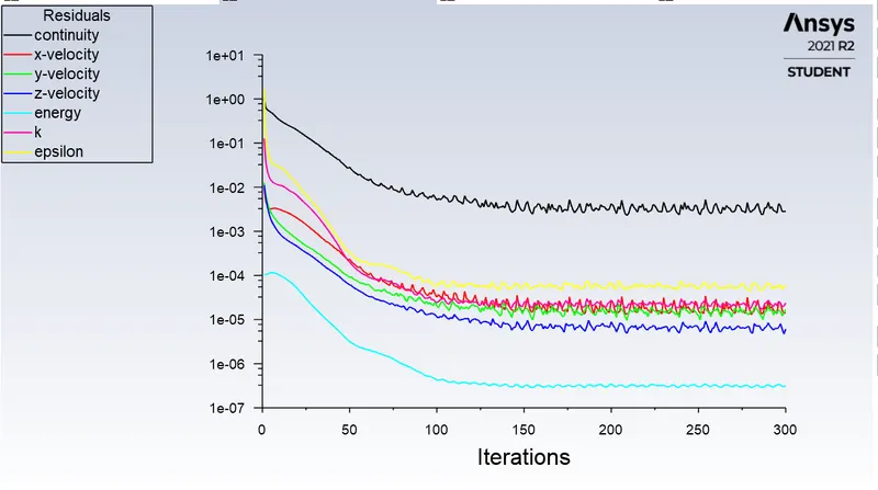
Residual plot:

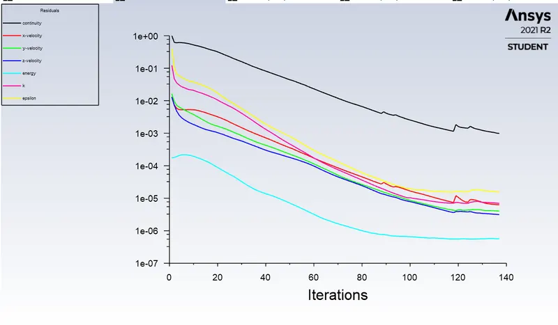
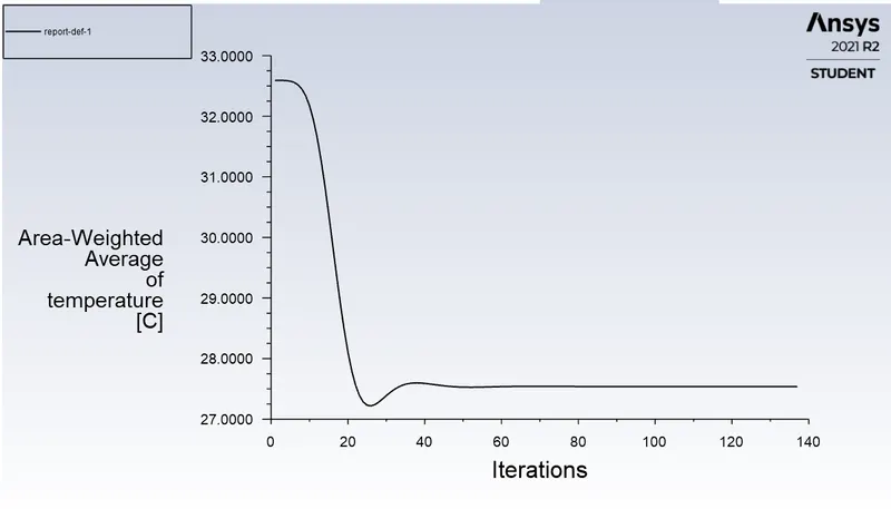
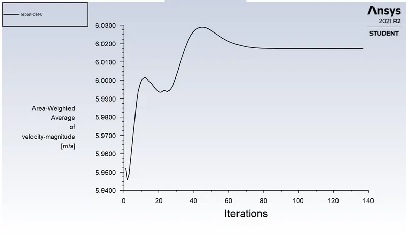
It converges after 140 iterations.

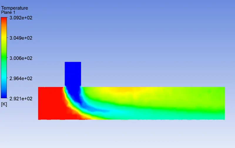
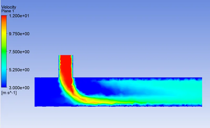
Temperature and velocity contour: Along pipe

Across pipe

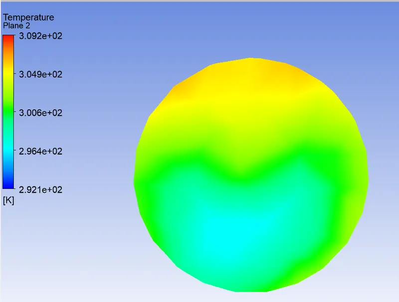
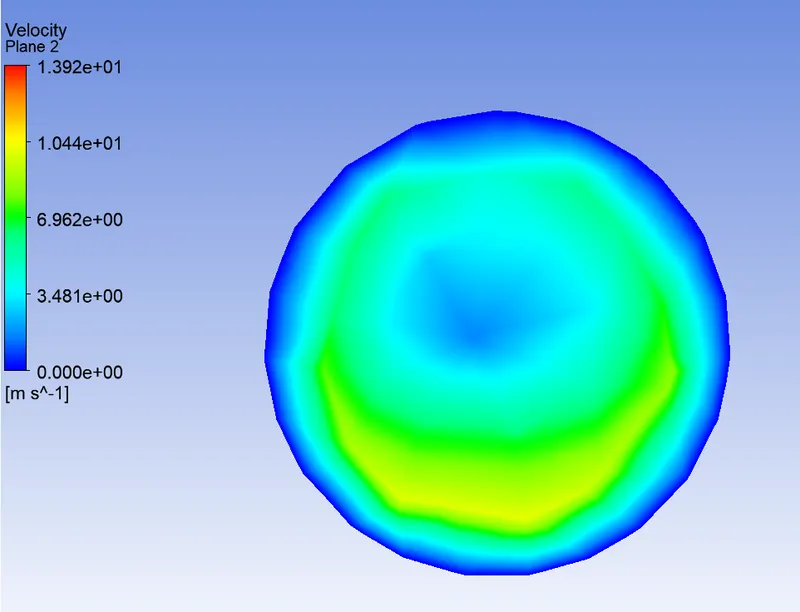
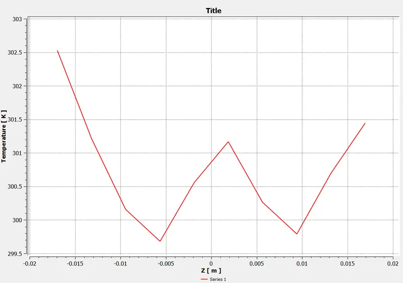
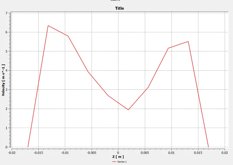
Line plots

a) Along pipe

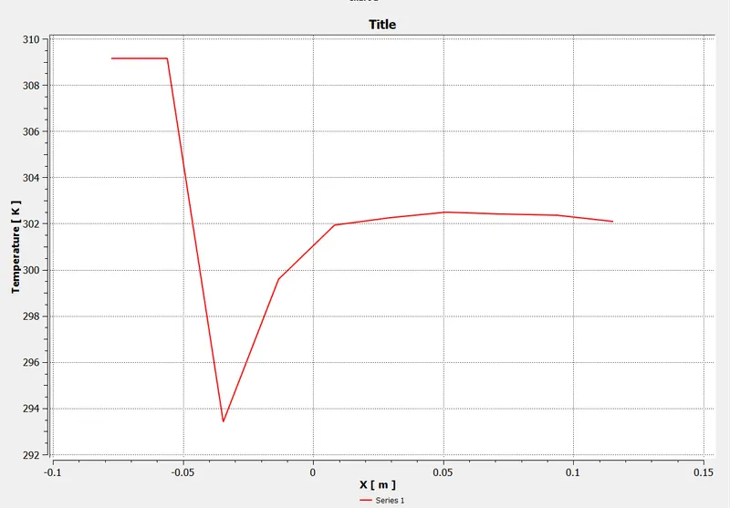
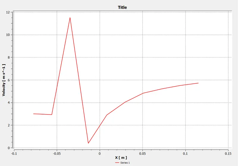
b) Across pipe

Case (2) Long Tee

i) Momentum ratio = 2

inlet_hot_velocity = 3 m/s

inlet_cold_velocity = 3*2 = 6 m/s

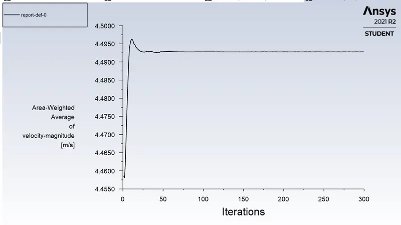
Contours :

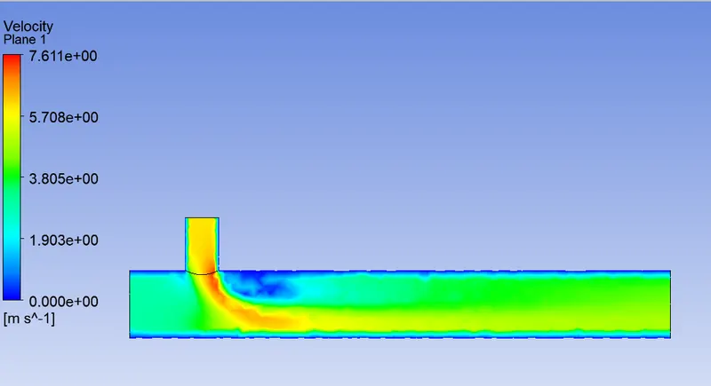
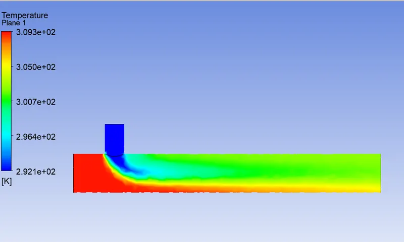
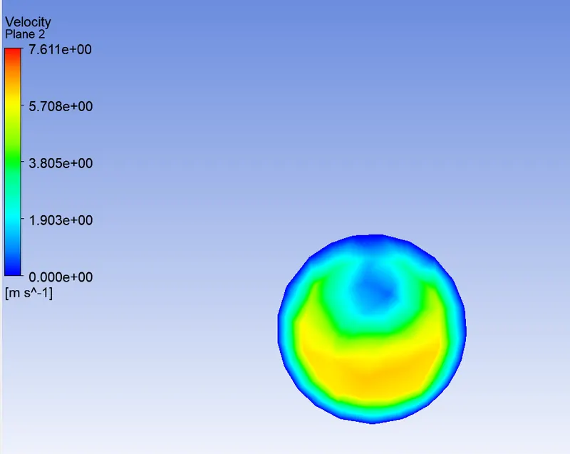
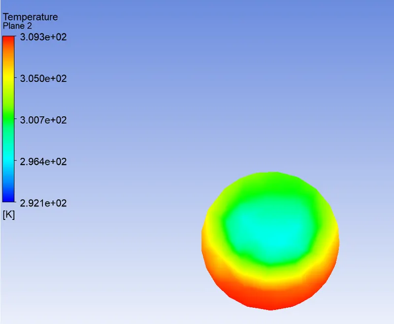
Case (2) Long Tee

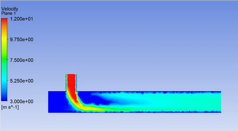
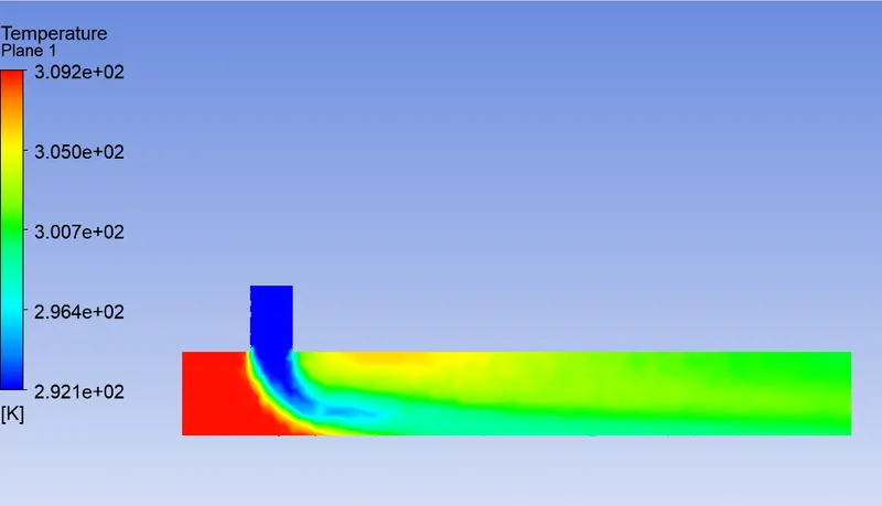
i) Momentum ratio = 4

inlet_hot_velocity = 3 m/s

inlet_cold_velocity = 3*4 = 12 m/s

Mesh independence study:

It is done to minimize simulation time. If output results are not changing after increasing the mesh elements, then its not necessery to fine tune mesh. So we use minimum no. of elements. It is done for momentum ratio 2 for short pipe.

No. of elements Outlet temp. (C)

12363 30.24725

15869 30.28915

19665 30.59952

So after 12363 elements, the results are not changing, so we can conclude we can keep 12363 elements in the study.

Also, k-Epsilon predicts the flow far from the wall. k-omega predicts flow near the wall. In our case, we are more interested in flow away from wall, hence we select k-Epsilon model for simulation.