Week 1- Mixing Tee

Objective:- To set up steady-state simulations to compare the mixing effectiveness when hot inlet temperature is 36⁰C & the Cold inlet is at 19⁰C.

Use the k-epsilon and k-omega SST model for the first case and based on your judgment use the more suitable model for further cases. Giving the reason for choosing a suitable model is compulsory.

1. Case 1
• Short mixing tee with a hot inlet velocity of 3m/s.
• Momentum ratio of 2, 4.
2. Case 2
• Long mixing tee with a hot inlet velocity of 3m/s.
• Momentum ratio of 2, 4.

Momentum ratio = velocity at cold inlet / velocity at hot inlet

In a table, compare the following values from the 2 cases.

1. Cell count
2. Average outlet temperature
3. Number of iterations for convergence

Expected results:

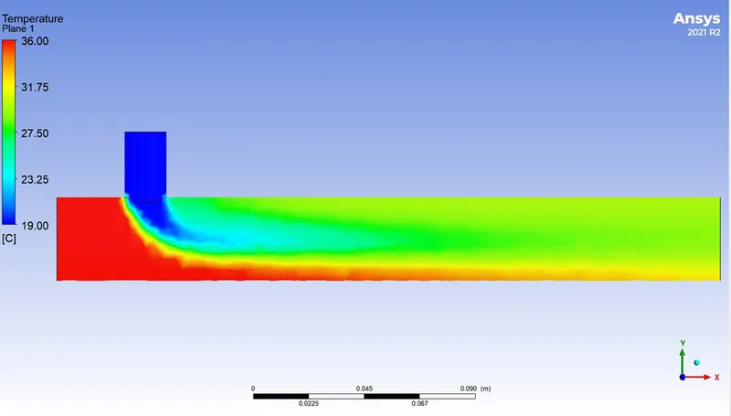
1. Velocity and temperature contour plots on the cut planes along and across the pipe.
2. Velocity and temperature line plots along and across the length of the pipe.
3. Perform Mesh independent study for any one case.
4. Discuss the effect of length and momentum ratio on results.

For each simulation, you need to show the convergence plot

Procedure:-

Case 1- Short mixing tee with Momentum ratio 2

Setup of the model

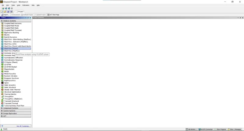
Select the ‘Fluid Flow (Fluent)’ model in Ansys Workbench

Drag the model to Project Schematic page.

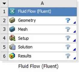
We can see the following options

1. Geometry

In this we will select the required file and setup the geometry

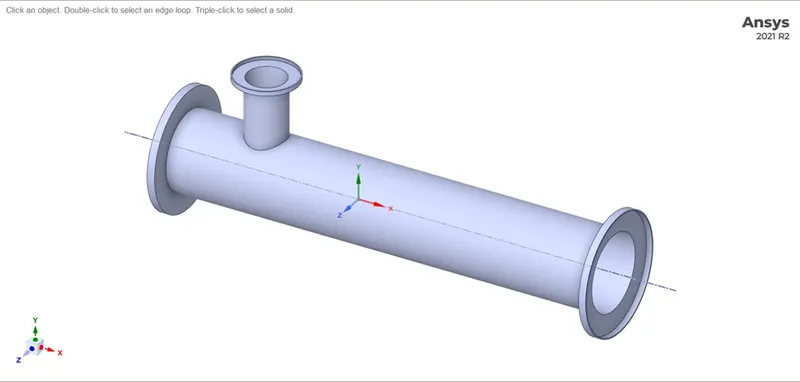
After setting the Geometry go for Volume Extraction option, since we are interested only in the volume through which the fluid flows

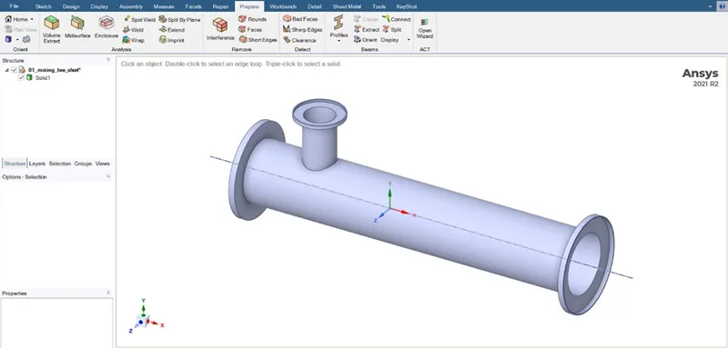
Select all the edges that covers the entire volume. In this case there are three edges

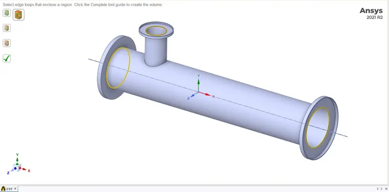
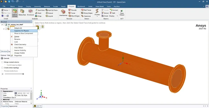
After Extraction of the required volume, select the solid part as shown below and select the option ‘suppress for physics’. So that part of the geometry is not considered in meshing

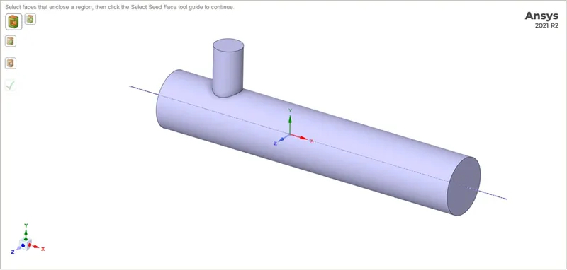
Below is the extracted volume of the model

2. Mesh

After setting the Geometry, close the window and then start the meshing of the model

Before meshing the model, it is better to give names to all the parts in the model. To do that, press ‘ctrl + F’ to select faces. Now select the face and right click on the selected face. We can see an option called ‘Create Named Section’. This option allows us to name the selected face

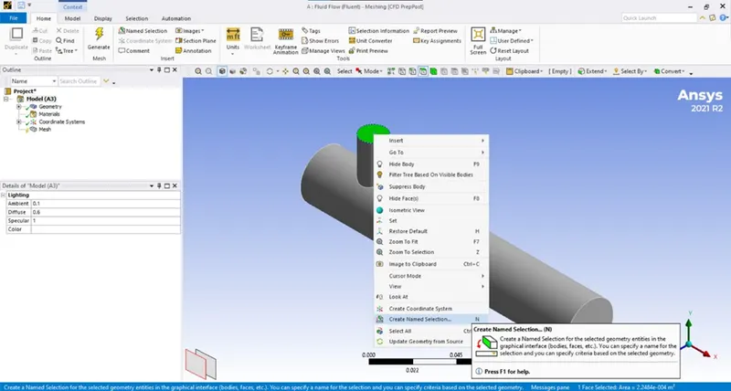
Below is the name given to each face. The fluid entering from y-direction is named as ‘inlet_cold_y’ and so on.

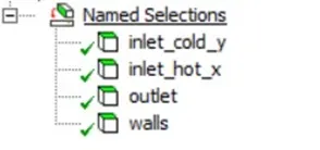
Once the naming of the model is done, we can proceed to the meshing part.

Right click on Mesh and click ‘Generate Mesh’ option.

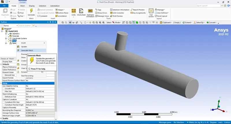
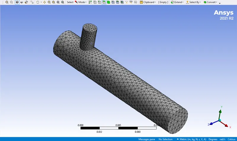
After this the Fluent software uses an algorithm to compute the mesh. Below is the meshed model

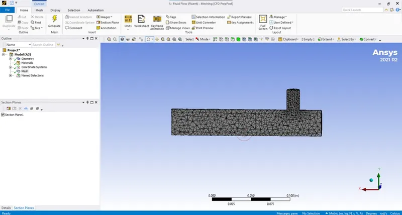
To make sure that our solid model is completely meshed, select the ‘section plane’ option and slice the model in half by drawing a line.

Below is the image of the model

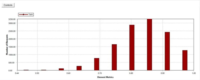
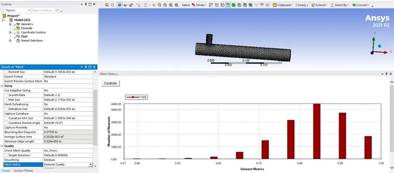
We can perform a quality check of the model. The quality ranges from 0-1. It can be seen that majority of the elements are more towards 1, i.e our mesh quality is good

3. Setup

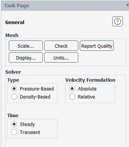
Now proceeding towards the model setup. Select the Solver type as Pressure-based, Velocity formulation as Absolute and Time as Steady under the General option

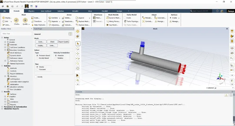
After that perform a Mesh check for any errors

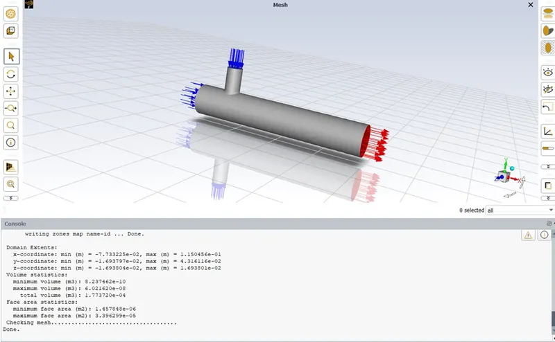
Now we will setup the Model. First click on ‘Physics’ option to setup the physical condition of the model. Since we are interested in tracking the Temperature we will tick the ‘Energy’ option.

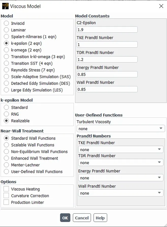
In our case the flow can be turbulent, so under ‘Viscous Model’ select the appropriate option as needed. Selecting the ‘k-epsilon’ type model for this case. Under ‘k-epsilon Model’ selecting ‘Realizable’ option which is an improved version.

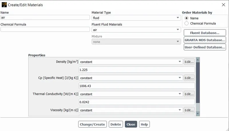
Now proceeding towards to create the material. Under ‘Physics’ option we can see there is an option ‘Materials’. In this case we will select ‘air’ as the material.

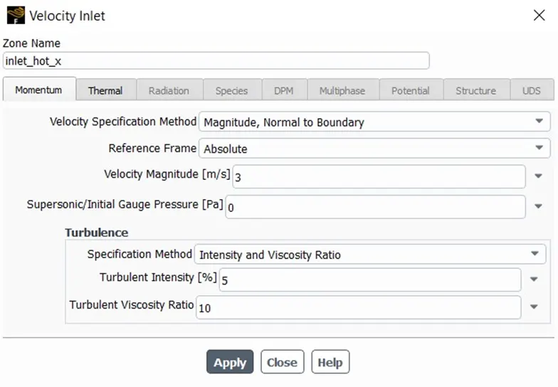
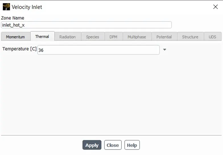
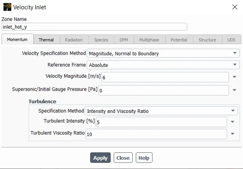
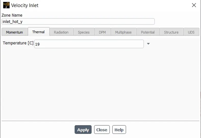
Now we will setup the boundary conditions. To do this click the ‘boundaries’ option under ‘zones’ and the below window will pop-up. After providing the Velocity and Temperature to both the inlets we will close the window.

Velocity of hot inlet

Temperature of hot inlet

Velocity of cold inlet

Temperature of cold inlet

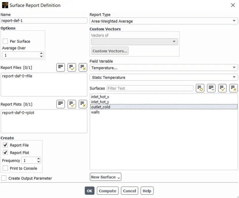
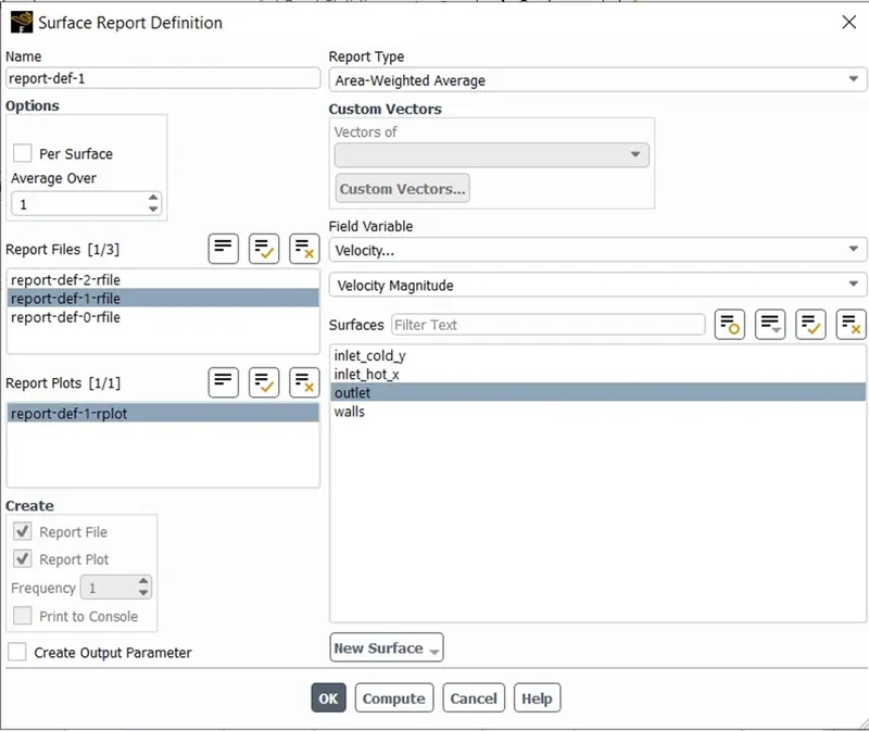
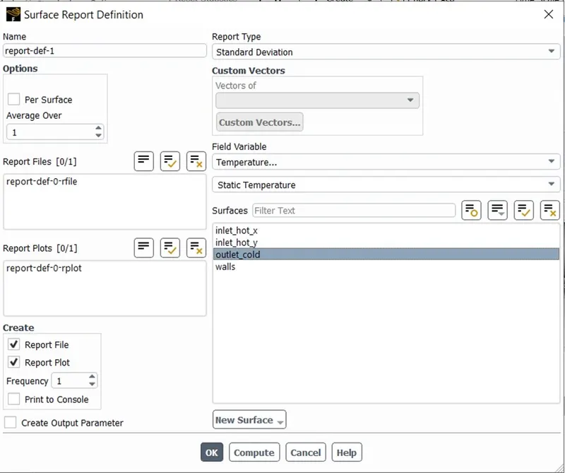
To track temperature and velocity and also standard deviation from the actual value we will select ‘Definition’ from ‘solution option and will create a ‘surface report’ for Temperature and Velocity.

Area-weighted average of temperature

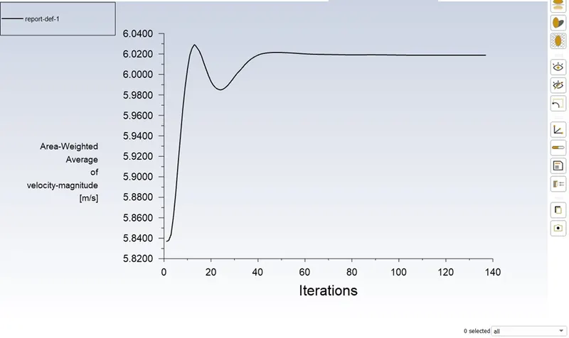
Area weighted average of velocity

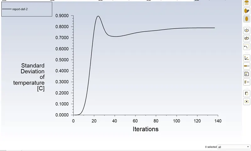
Standard Deviation

After this now we will initialize the problem. To do this select ‘Initialize’ option under ‘Solution’ tab. After the problem has been initialize, we will provide the number of iterations and hit on calculate.

4. Results

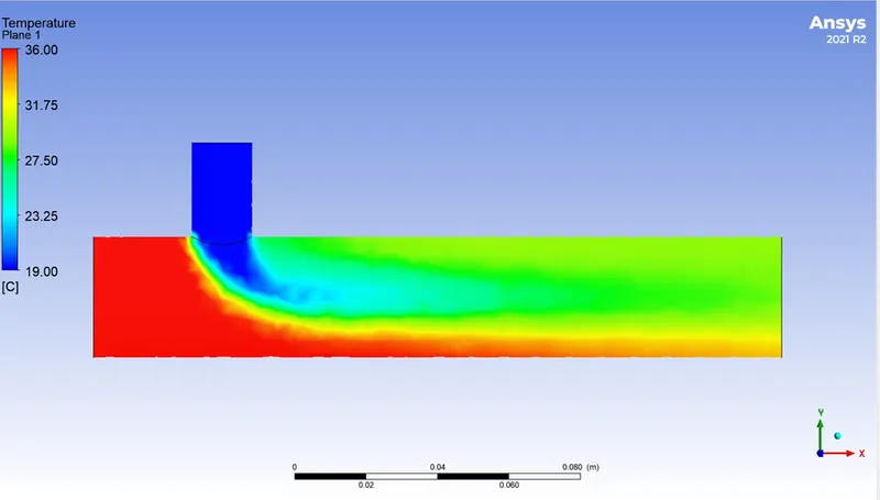
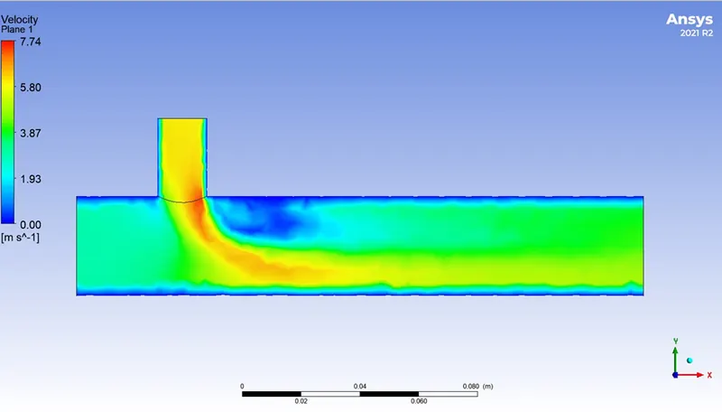
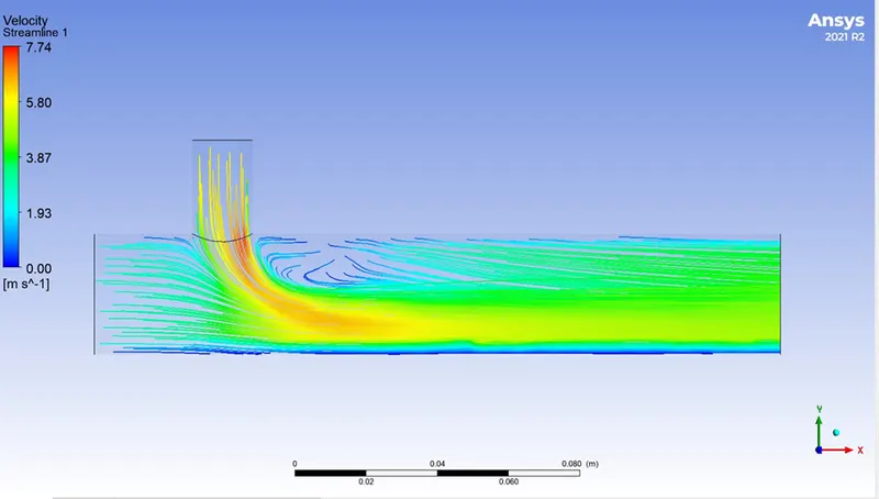
Once the software computes the calculations, we will close the window and select the last option i.e ‘Results’. We can view the results of the Temperature and Velocity as seen below

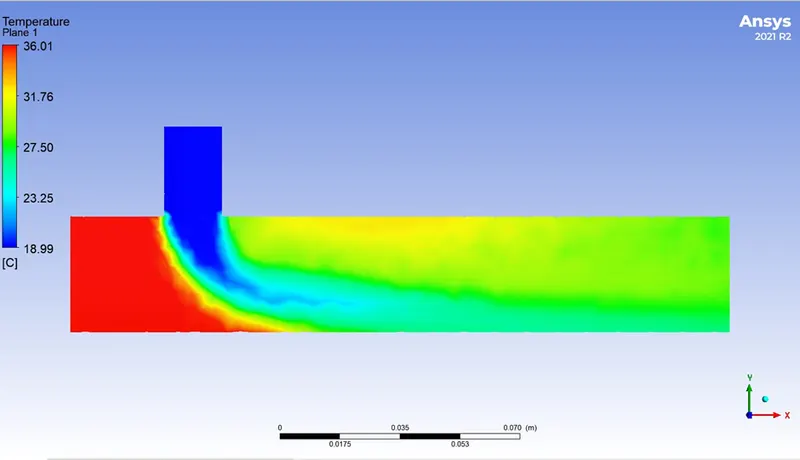
Contour plot of Temperature

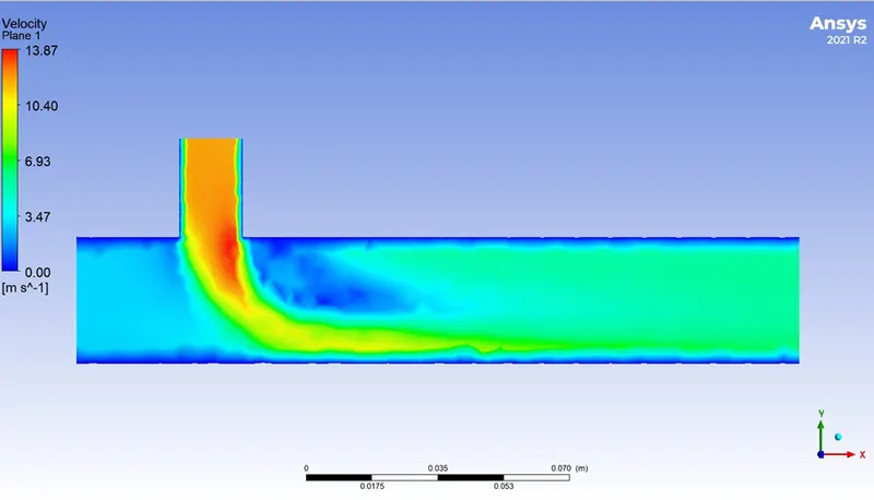
Contour plot of Velocity

Line plot of Velocity

Line plot of Temperature

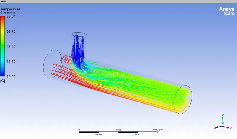
Temperature Variation across the pipe

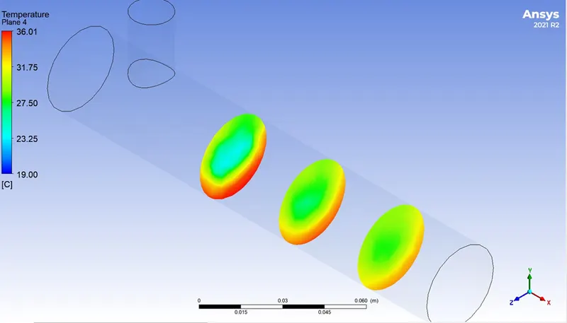
Velocity variation across the pipe

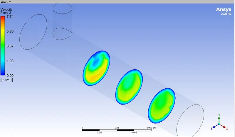
Comparison of k-epsilon and k-omega SST model

Number of Iterations

k-epsilon model

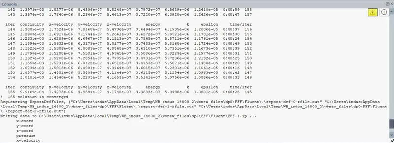
k-omega SST model

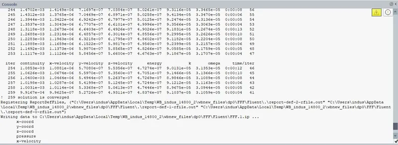
It can be clearly seen that the k-epsilon model took 155 iterations to converge and the k-omega SST model took 259 iterations for convergence

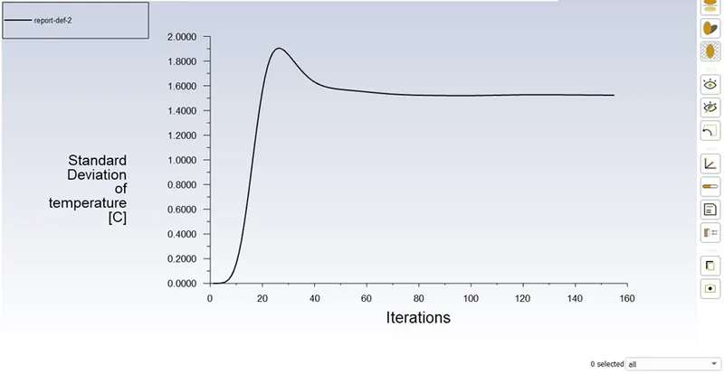
Standard deviation of temperature

Below are the plot for k-epsilon and k-omega SST model

k-epsilon Standard Deviation of Temperature

k-omega Standard Deviation of Temperature

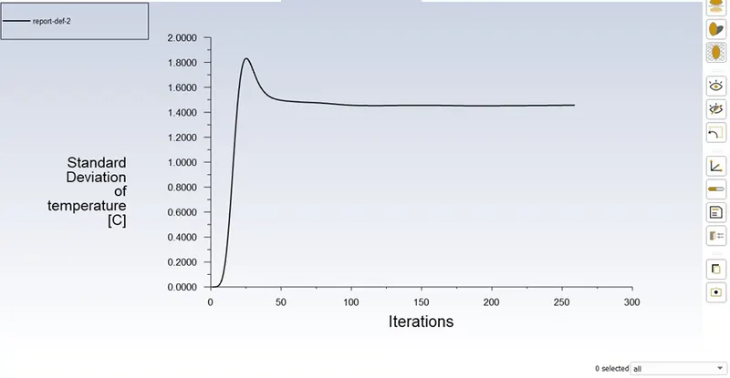
Here we can observe that the standard deviation of k-epsilon is around 1.5 whereas the standard deviation of k-omega SST is below 1.5 i.e around 1.4

Standard deviation is a mathematical tool to help us access how far the values are spread above and below the mean. A high standard deviation shows that the data is widely spread (less reliable) and a low standard deviation shows that the data are clustered closely around the mean (more reliable).

Temperature plots

k-epsilon model

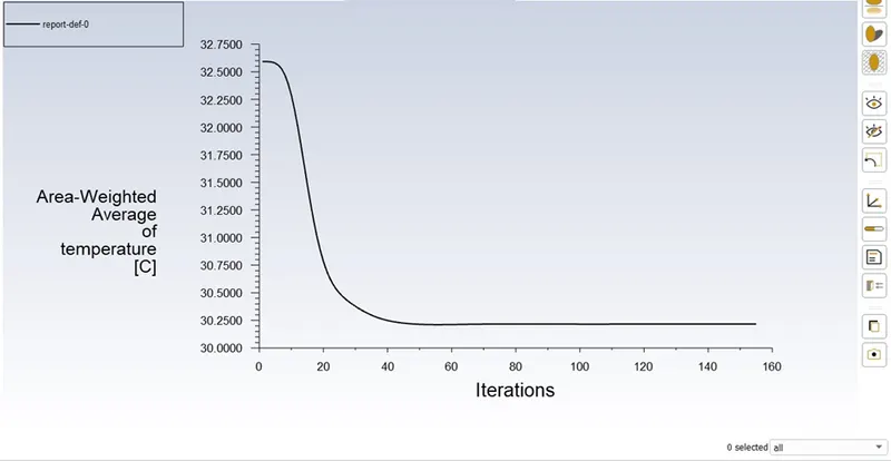
If we observe closely then we can see that the Area-Weighted Average of Temperature is somewhat below 30.25 C

k-omega SST model

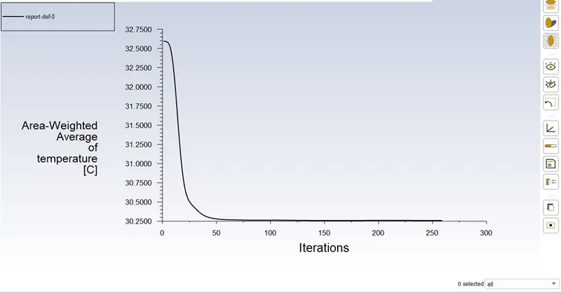
Whereas in this case the Area-Weighted Average of Temperature is exactly 30.25 C

Velocity Plot

k-epsilon model

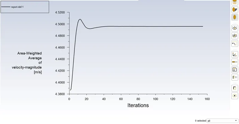
k-omega model

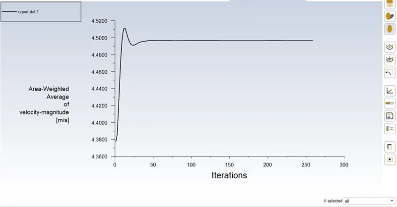
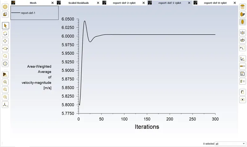
It can be seen that no change is observed in the Area-Weighted Average of Velocity-magnitude plot for both k-epsilon and k-omega SST model.

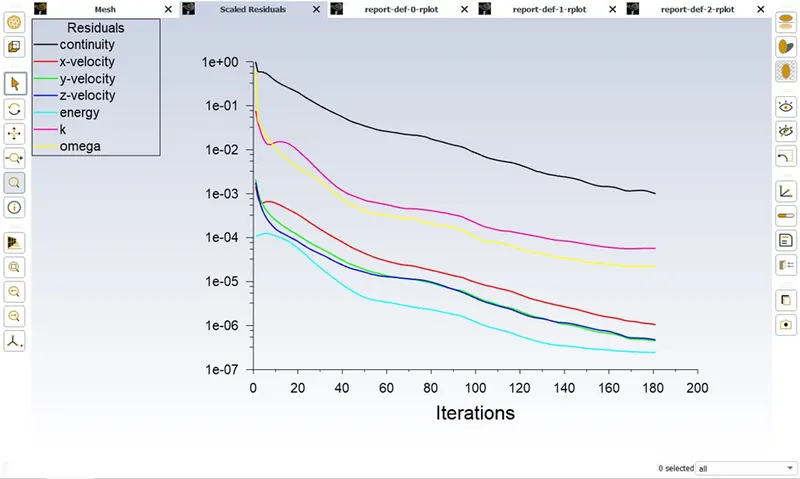
Residuals

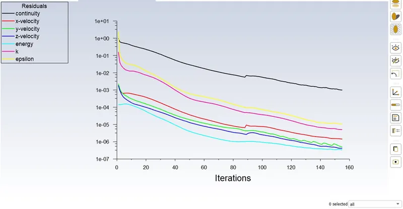
Residuals are the differences in the value of a quantity between two iterations. This means that the more the residual is low the less the results will change if you will continue to iterate.

k-epsilon model

k-omega SST model

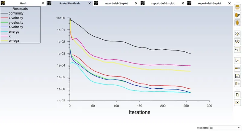
No change is observed in the above two plots.

Conclusion:- Both the model gives almost the same results. The difference is that the k-epsilon model took less number of iterations to converge than the k-omega SST model. Also if we observe a bit closely, the standard deviation of the k-omega SST model is less than the k-epsilon model

So for further analysis we will be using the k-omega SST model.

Case 1- Short mixing tee with Momentum ratio 4

Everything will be same as mentioned above. The only difference will be setting up of the boundary conditions for the velocity of cold inlet. In this case the velocity of the cold inlet will be 12 m/s

Number of iterations to converge

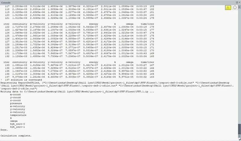
Plots

Residuals

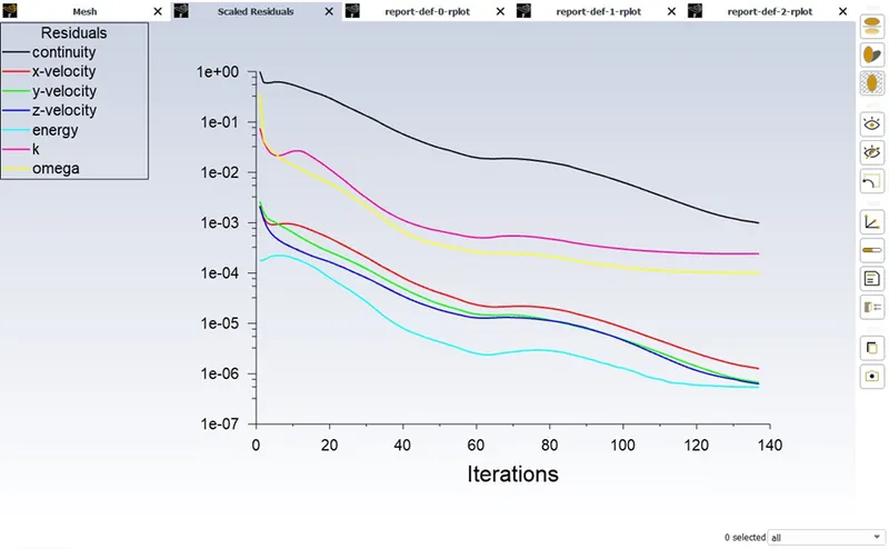
Temperature plot

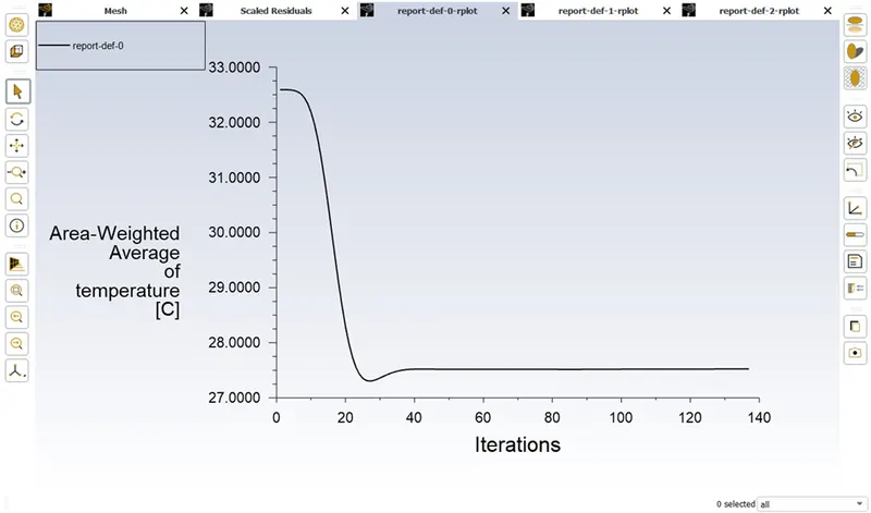
Velocity plot

Standard Deviation

Results:-

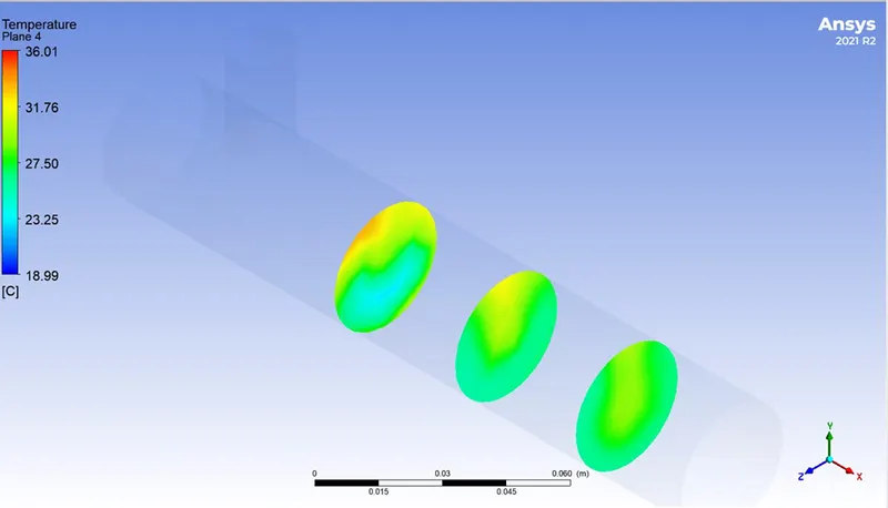
Contour plot of Temperature

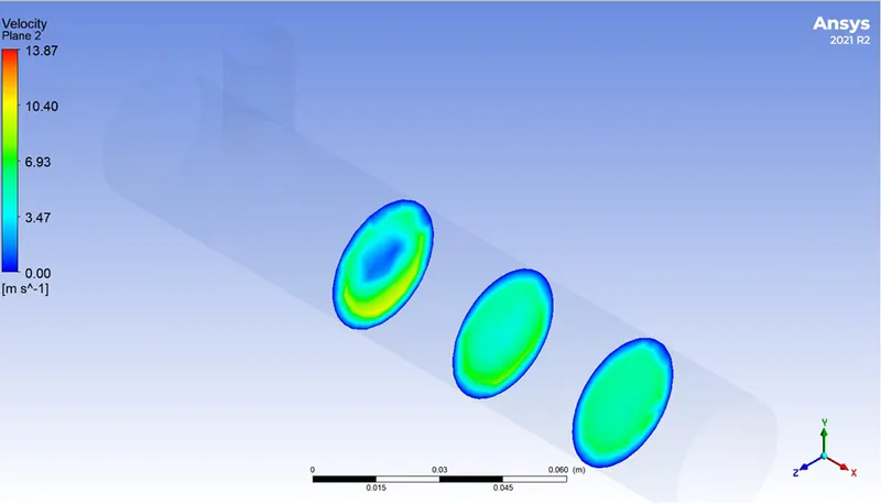
Contour plot of Velocity

Temperature across the pipe

Velocity across the pipe

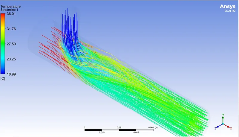
Line plot of Temperature

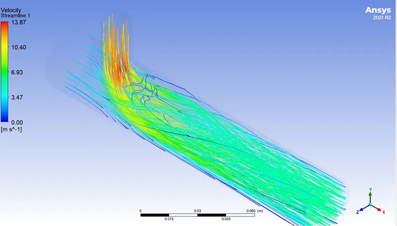
Line plot of Velocity

Case 2- Long mixing tee with Momentum ratio 2

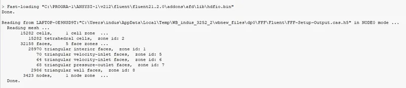
Number of Cells

Quality of Mesh

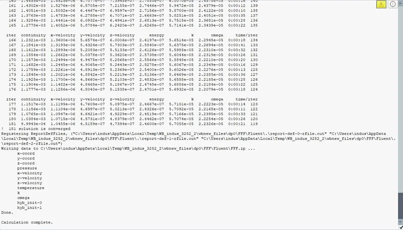
Number of Iterations to converge

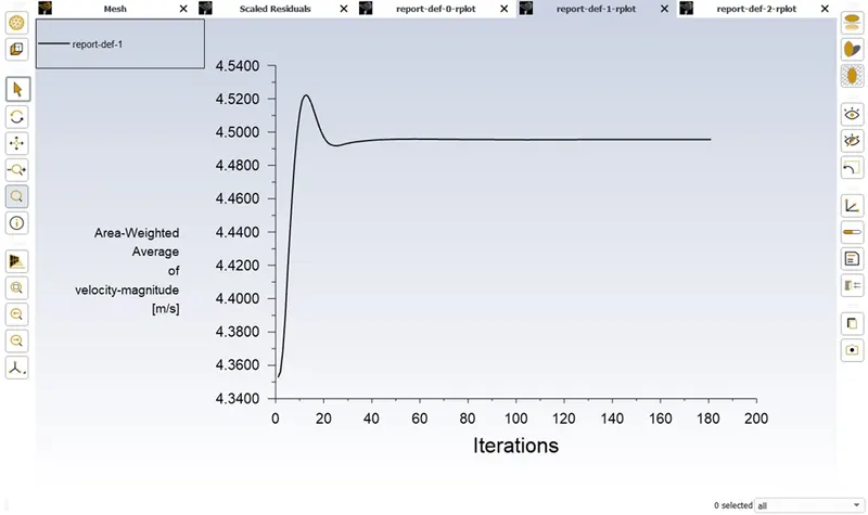
Plots

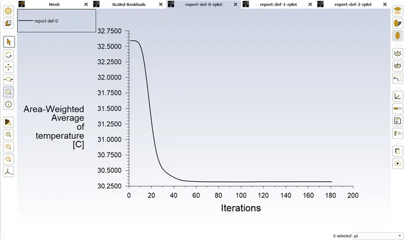
Temperature plot

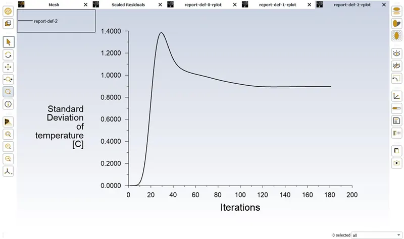
Standard Deviation

Residuals

Velocity plot

Temperature contour plot

Velocity Contour plot

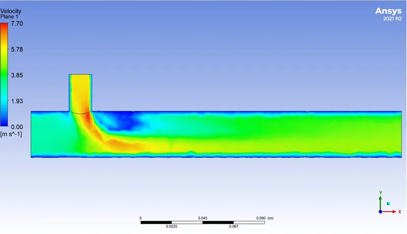
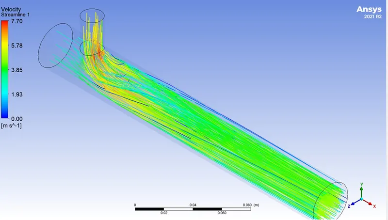
Temperature line plot

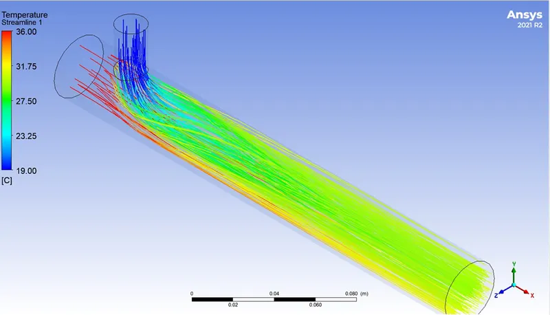
Velocity line plot

Temperature variation across the pipe

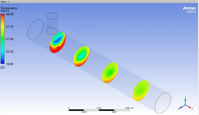
Velocity variation across the pipe

Case 2- Long mixing tee with Momentum ratio 4

Plots

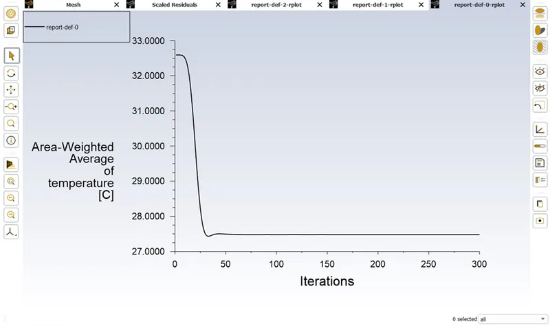
Temperature plot

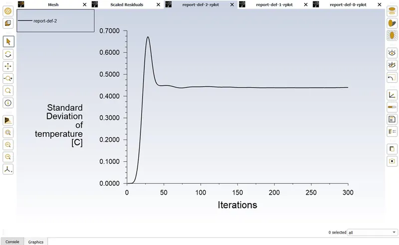
Standard Deviation

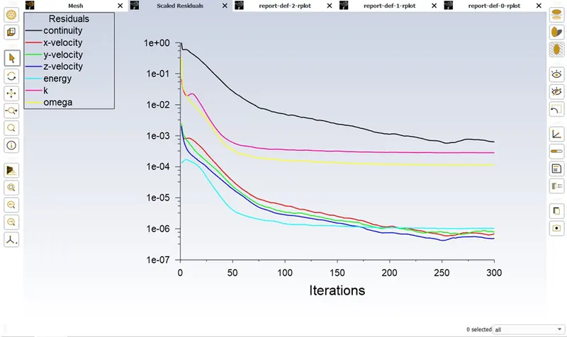
Residuals

Velocity plot

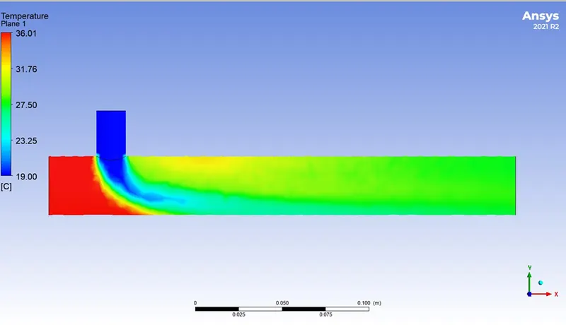
Temperature contour plot

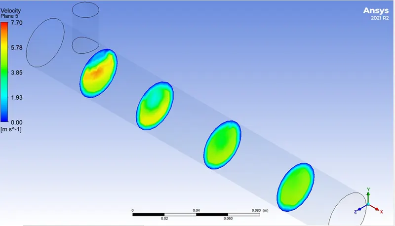
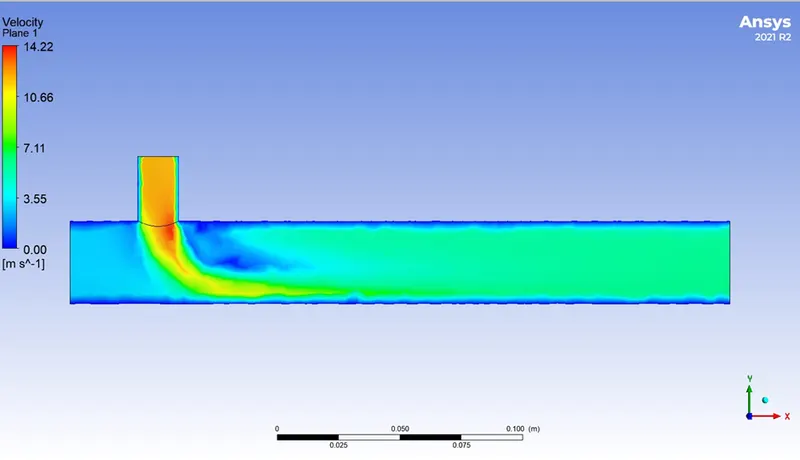
Velocity contour plot

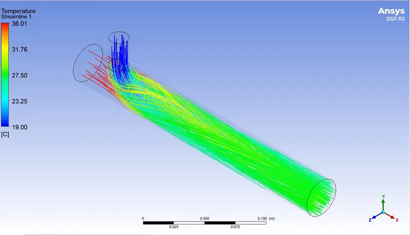
Temperature line plot

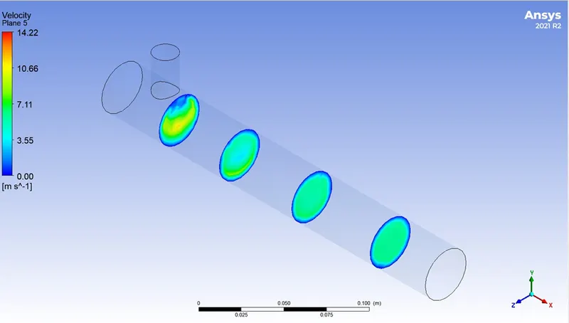
Velocity line plot

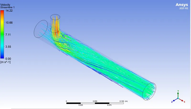
Temperature variation across the pipe

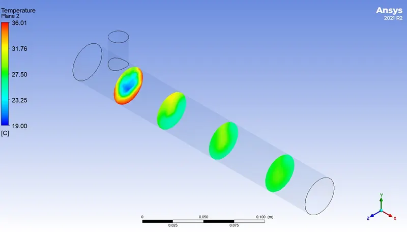
Velocity variation across the pipe

Comparison table

	Cell count	Average outlet temperature	Number of Iterations for convergence
Short Tee	12444	30.25	259
Long Tee	15282	30.30	181

Mesh Independence Study for short tee mixing with momentum ratio 4

Here we will change the element size to almost 0.001, so that we have a more refined mesh. Below is the image of the finer meshed model

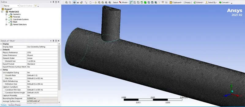
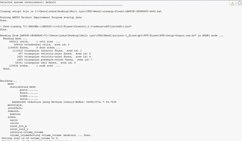
After meshing this we can see that the number of cells is 569312 which is very large. The governing Fluid Dynamics equations are solved for each and every cell. The more the number of cells the more equations are there to solve and hence more the computation time. The computational time does not has a linear relationship with the increase in the cell value

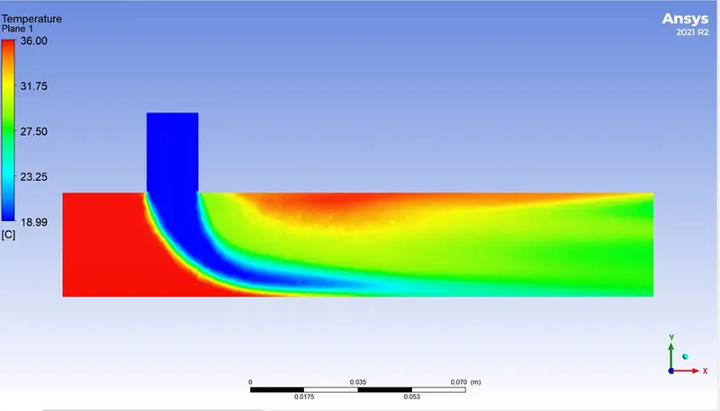
Temperature contour plot

Velocity contour plot

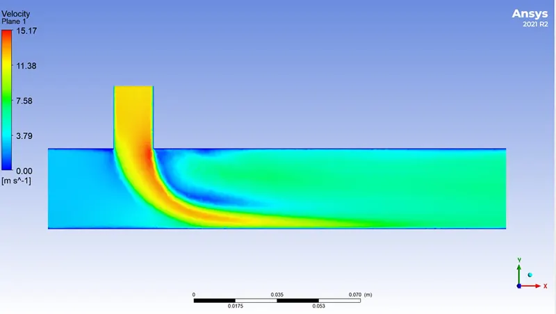
In the above plots we can see that the Temperature and Velocity distribution are very much sharp. This is called as mesh refinement.

Also we can observe that there is almost no change in the temperature of the fluid at the outlet. It is concluded that by increasing the number of elements, there is no change in the temperature at the outlet. The only difference is that it takes more amount of computational time.

Conclusion:-

Effect of length and momentum ratio on results

Since the temperature at the outlet does not vary that much for short and long tee mixing, its only the velocity of the fluid that determines the temperature of the fluid at the outlet.