Week 1- Mixing Tee

AIM:-To set up steady-state simulations to compare the mixing effectiveness when hot inlet temperature is 36 C & the Cold inlet is at 19 C.

INTRODUCTION:

Ansys Fluent is the industry-leading fluid simulation software known for its advanced physics modeling capabilities and industry leading accuracy.Ansys Fluent gives you more time to innovate and optimize product performance. Trust your simulation results with a software that has been extensively validated across a wide range of applications. With Ansys Fluent, you can create advanced physics models and analyze a variety of fluids phenomena—all in a customizable and intuitive space.

OBJECTIVE:

In this challenge we will be simulating a flow through tee joint where air at 36degree C will mix with air at 19 degree C. We have 4 cases for this.
1.Finding out which method k-epsilon or k-omega is better at giving best results.
2.Flow through short pipe at hot air at 3m/s and cold air at 6 m/s.
3.Flow through short pipe at hot air at 3m/s and cold air at 12 m/s.
4.Flow through long pipe at hot air at 3m/s and cold air at 6 m/s.
5.Flow through long pipe at hot air at 3m/s and cold air at 12 m/s.

WE WILL BE PROVIDING THE BELOW RESULT FOR EACH CASE:

1. Velocity and temperature contour plots on the cut planes along and across the pipe.
2. Velocity and temperature line plots along and across the length of the pipe.

AFTER PERFORMING THE ABOVE EXPERIMENTS WE WILL BE PROVIDING A MESH
INDEPENDENT STUDY TO SHOW THE EFFECT OF MESH SIZE ON THE SOLUTION.

THEORY:

In a mixing tee a fluid with 2 different temperature are coming through two inlets and is getting mixed inisde a pipe and the effectiveness of mixing is evaluated on parameters like velocity of cold and hot fluid. Also we perform this study to reach optimum cooling and good mixing. Now let us see the general setup of the experiments. Let us see which viscous model shall we use k-epsilon or k_omega.

But first let us know what k-epsilon and k-omega is:-

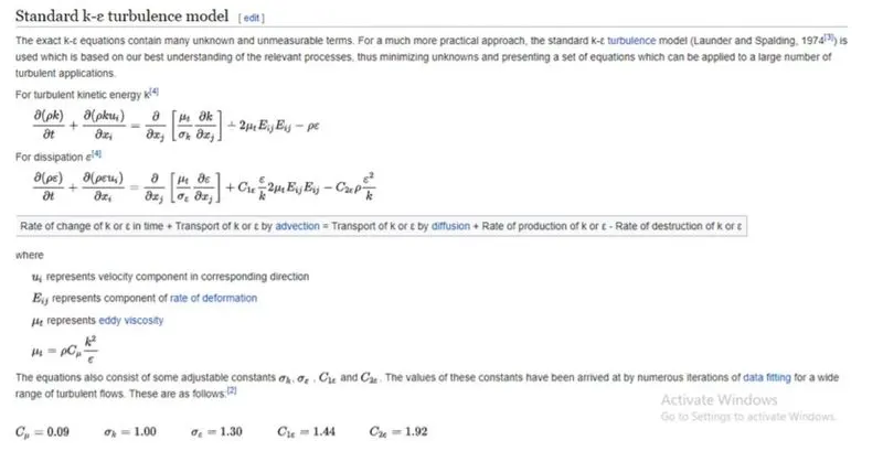
k-epsilon:

• K-epsilon (k-ε) turbulence model is the most common model used in CFD to simulate mean flow
  characteristics for tutbulant flow conditions. It is a two equation model that gives a general description
  of turbulence by means of two transport equations (PDEs). The original impetus for the K-epsilon
  model was to improve the mixing-length model, as well as to find an alternative to algebraically
  prescribing turbulent length scales in moderate to high complexity flows.
• The first transported variable is the turbulent kinetic energy (k).
• The second transported variable is the rate of dissipation of turbulent kinetic energy (ε).

k-omega:

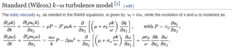
In computational fluid dynamics, the k–omega (k–ω) turbulence model is a common twoequation turbulence model, that is used as an approximation for the Reynolds-averaged Navier– Stokes equations (RANS equations). The model attempts to predict turbulence by two partial
differential equations for two variables, k and ω, with the first variable being the turbulence kinetic energy (k) while the second (ω) is the specific rate of dissipation (of the turbulence kinetic energy k into internal thermal energy).

PROCEDURE:

The SST k-omega model reduces to a standard k-epsilon model away from walls.
Near walls, the SST k-omega uses the the omega formulation whereas the realizable k-epsilon uses the epsilon formulation.
The two models differ in their approach both near walls and away from walls.
The SST k-omega model is generally thought to be better near walls, but because it reduces to the standard k-epsilon model away from walls and not the realizable k-epsilon model, it also has weaknesses.
The two models are very different and it should be no surprise that significant differences in results can be obtained from each model (this should be considered
the norm rather than unusual).

HENCE WE ARE USING THE k-epsilon TURBULANCE MODEL TO SOLVE THIS CHALLENGE.
SO LET US TAKE A LOOK AT THE COMMONALITIES OF THE SIMULATION STEP BY STEP.
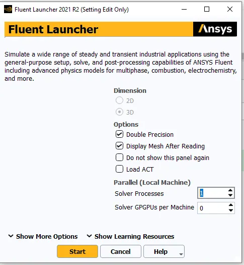
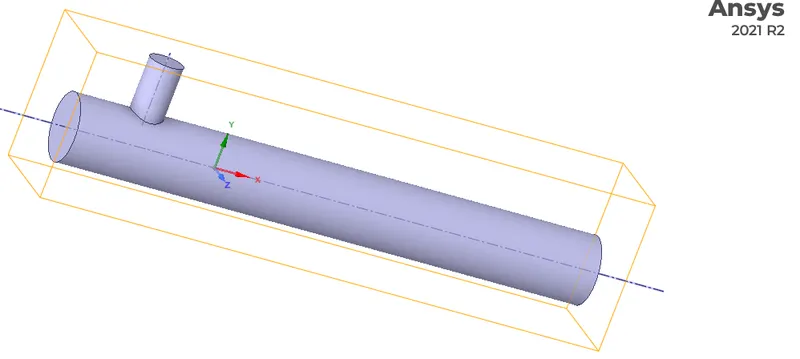
STEP 1: WE ARE PROVIDED WITH A STEP FILE OF MIXING TEE. FIRST WE HAVE TO IMPORT THE GEOMETRY INTOO ASNYS SPACECLAIM.
STEP 2: THEREAFTER WE HAVE TO EXTRACT THE VOLUME OUT OF THE SOLID OBJECT USING THE FOLLOWING TAB.

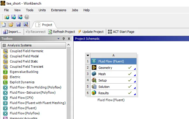
1. Click on Fluid flow(Fluent) in Ansys Workbench.

2. Now click on geometry to import mixing tee model. It will redirect to Spaceclaim, Ansys’s geometry model manipulator.

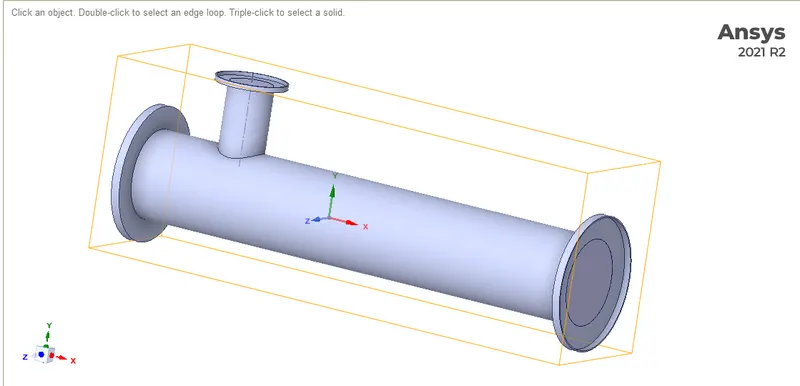
3. We are to analyse the mixing of two fluid, so there is role of parts other than two pipes. To supress that we need to extract volume of tee. Go to prepare menu and click on volume extract. Switch to edge selection and select three outer edges and click on green check button.

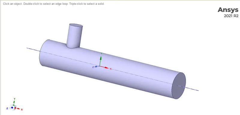
4. Hide solid by unchecking it from structure menu to see volume, which we have extracted. Supress solid by clicking on option supress for physics.

5. Exit from Spaceclaim and click on mesh to open mesh menu.

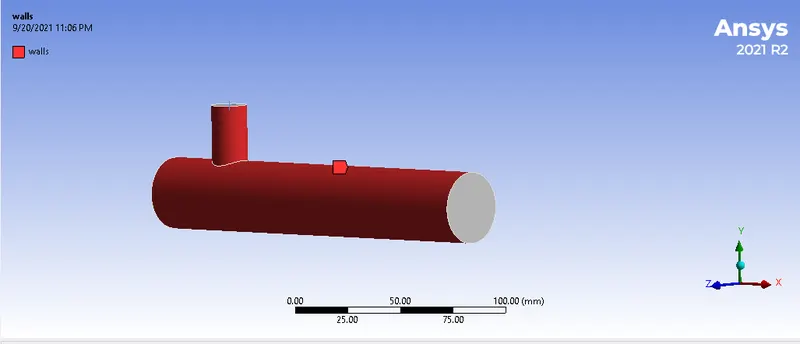
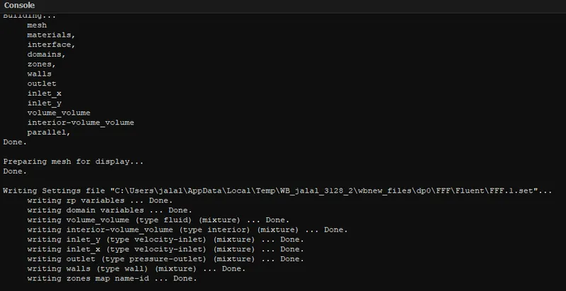
6. Select outer face and press right click of mouse, it will open a menu. Click on option create named selection and write suitable name for face.
Repeat for other faces.

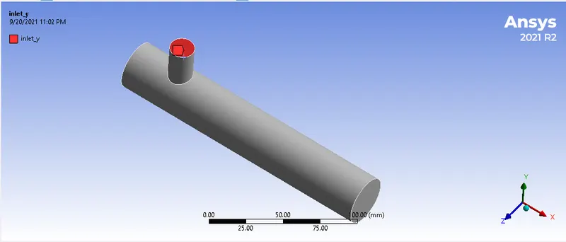
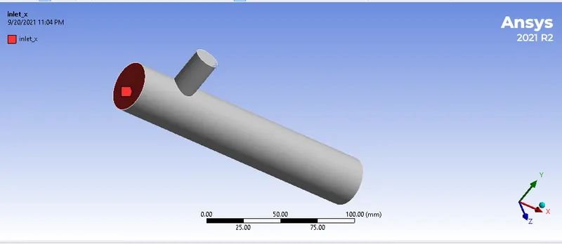
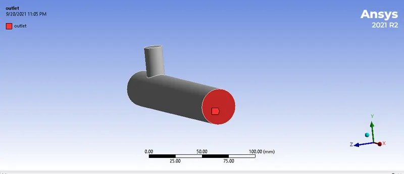
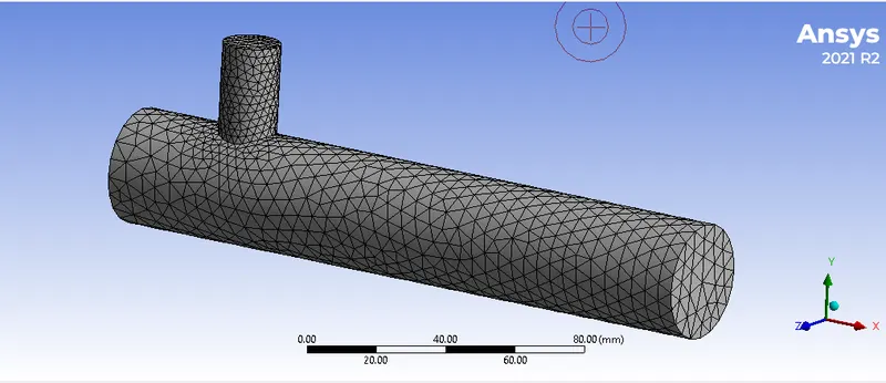
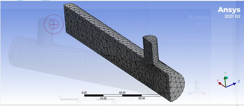
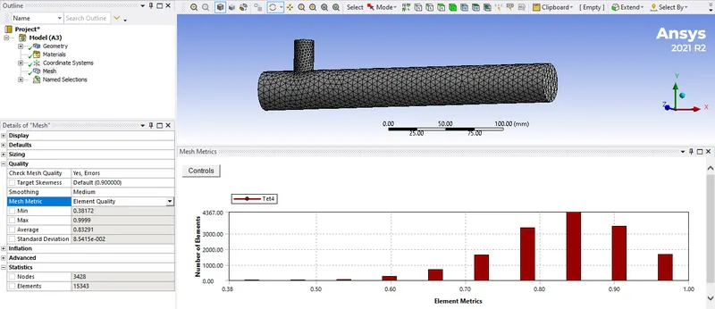
7. Now click on mesh option and choose generate mesh. It will generate mesh according to some predefined criteria. Element size can be selected but it is going to affect simulation time. Section plane can be created to see inner portion of geometry

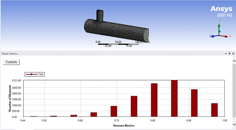
8. Select the option element quality to see, how many elements are defying quality. Quality is measured on the scale of 0 to 1. In our graph most of the element are near to 1 so we can say it is good quality.

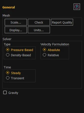
9. Exit mesh and open setup. First, Check mesh, it is throwing no error then only we can proceed further. We are going to do pressure based steady state simulation, so choose these options on task page.

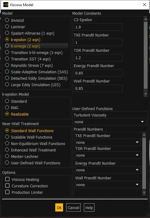
10. Go to physics menu and select viscous model. It will open a menu, choose realizable k-epsilon model and close it.

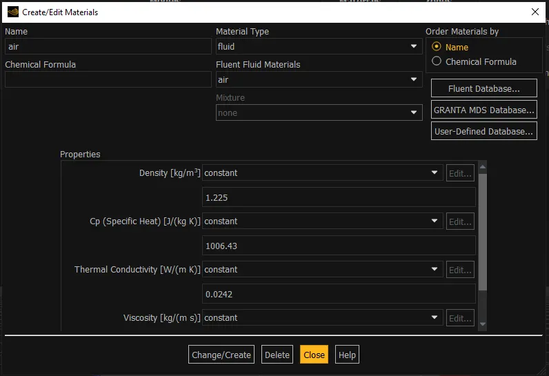
11. Click on material and choose air as working fluid. Check working fluid by clicking on cell zone conditions option, if it is air then proceed.

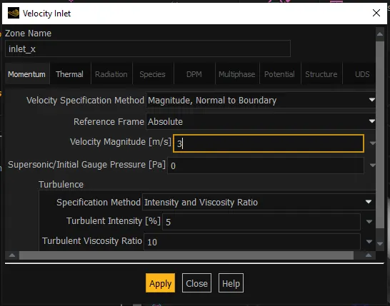
12. Now go to boundaries option to set boundary conditions. Select inlet_x and click on option edit. It will open a menu, where all the parameter can be set whether it is thermal, radiation, momentum etc. Put the value of velocity as 3m/s and go to thermal parameter to set temperature as 36C, for hot fluid.

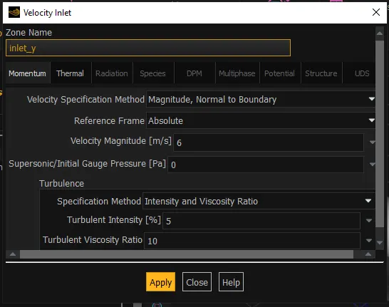
13. Repeat the same procedure for cold fluid coming, velocity –6 m/s, temperature – 19C.
14. We want to generate temperature report of outlet and we want standard deviation of temperature also. Go to solutions tab and select
definition and select area weighted average. In the opened menu select temperature as field variable. Similarly select standard deviation in
definitions menu.
15. Now click on initialization to calculate approximate values of velocity and pressure.
16. Change the number of iterations to 250 and click on calculate. If solution is not converged, then iterations can be increased.
17. Exit setup and double click on result to open CFD post. Check boxes to see walls and other parts. Click on walls and go to render set
transparency of 0.4 to inside of wall. Colour can also be changed to white for clear visibility.
18. Now insert a XY plane in wall by clicking on plane in location option of insert.

19. Go to colour of plane and change it by variable choose option temperature. Similarly, velocity contours can be created by just changing
variable as velocity.
20. Right click on plane which we created and select streamline. Go to appearance and select temperature to see plot line on plane. Similar
procedure can be repeated for velocity plot line

RESULTS:
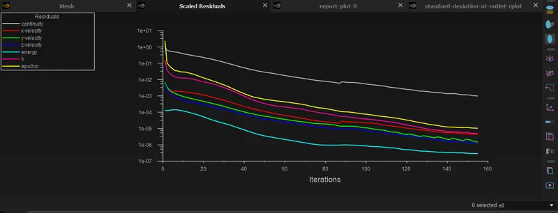
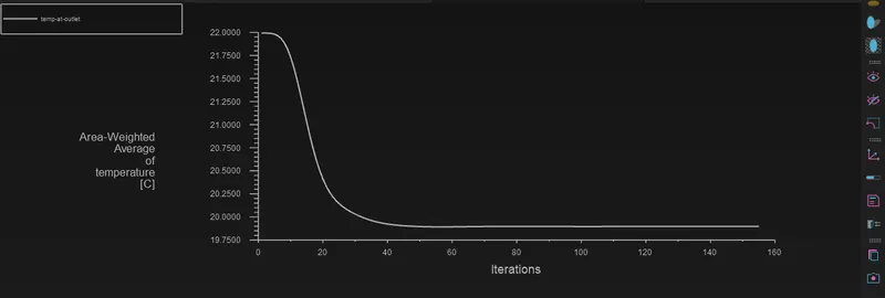
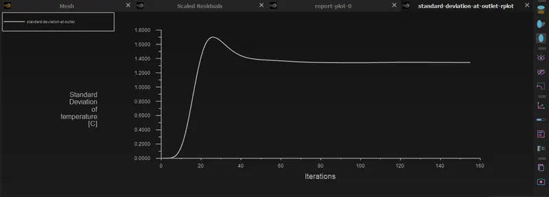
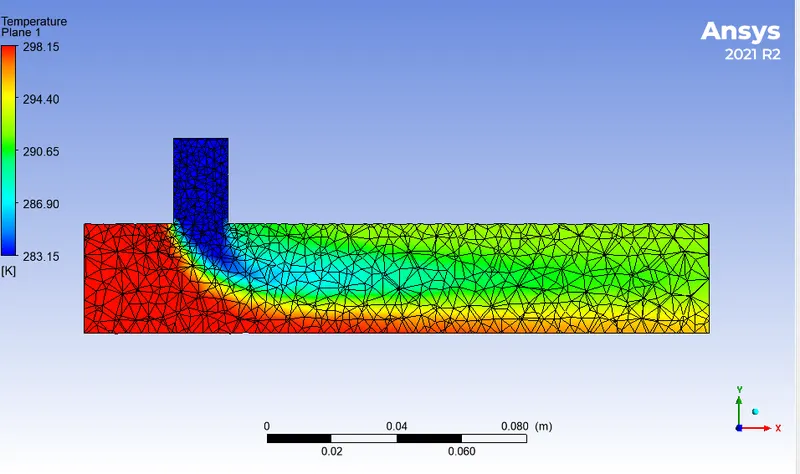
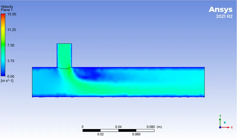
CASE1: In this short mixing tee is used, which was mixing two fluid with temperature 6C and 19C. Velocity of hot fluid was 3m/s and cold fluid was 6m/s. we used two different turbulent solvers for it first was realized k-epsilon and second was k-omega SST. The k-epsilon is giving better results because solution was converged after few iterations

Plot and contours from k-epsilon model:

Residuals:

Average Temperature vs Iterations:

Standard Deviation of Temperature vs Iteration:

Temperature contour:

Velocity contour:

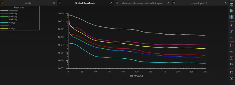
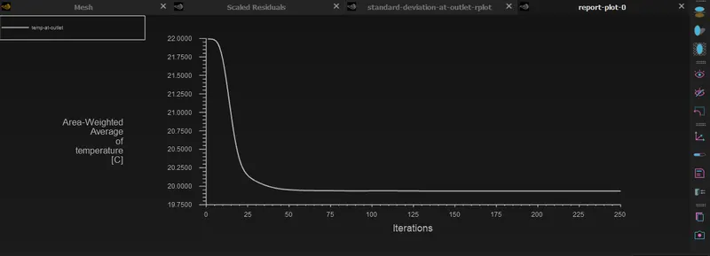
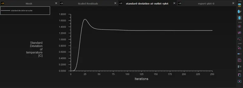
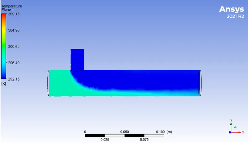
Plot and contours from k-omega model:

Residuals:

Average Temperature vs Iterations:

Standard Deviation of Temperature vs Iteration:

Temperature contour:

Velocity contour:

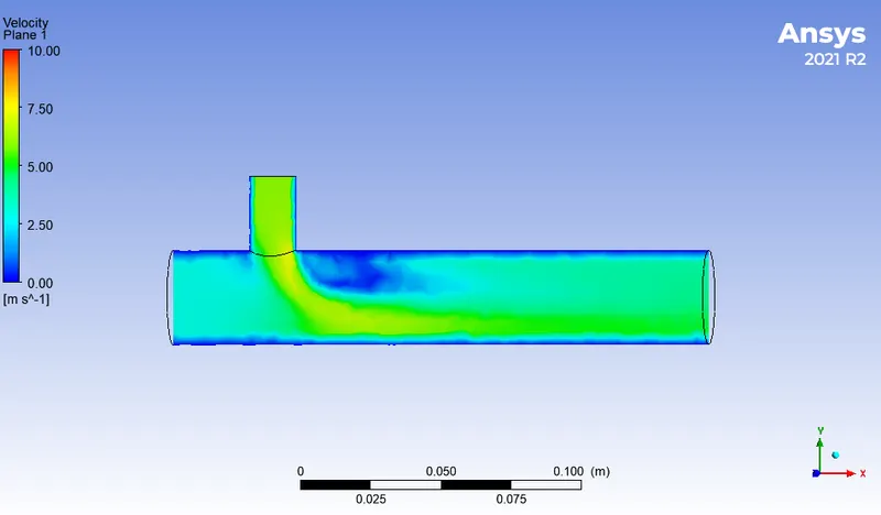
Table:-

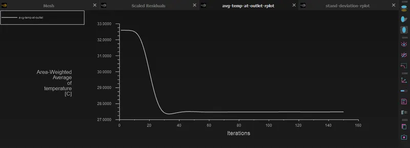
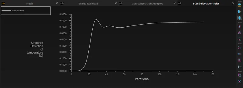
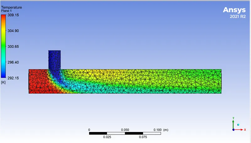
CASE2: In this case long mixing tee is used, which was mixing two fluid with temperature 36C and 19C. Velocity of hot fluid was 3m/s and cold
fluid was 12m/s.

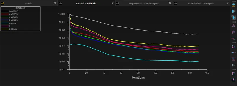
Residuals:

Average Temperature vs Iterations:

Standard Deviation of Temperature vs Iteration:

Temeprature Contour:

Velocity Contour:

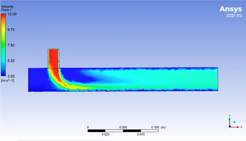
table:

THE GREATER THE LENGTH OF PIPE RESULTS IN BETTER MIXING.
HIGER THE MOMENTUM RATIO BETTER IS THE VOLUME FLOW RATE HENCE GREATER AMOUNT OF COLD AIR GETS MIXED WITH THE HOT FLUID TO
ACHIEVE EFFECTIVE COOLING.

CONCLUSION:

Hence from this challenge we have learnt the following:-
1.Longer length of pipe increases effectiveness of mixing.
2.Greater momentum ratio of cold air achives effective cooling.
3.Mesh size is important for generating accurate results.
4.We have seen various methods to visualize the temperature and velocity change through the TEE and at OUTLET.

• k- epsilon model predicts well far from the boundaries (wall) and k- omega model predicts well near the wall. Even though it depends on Y+. Therefore, K-epsilon model is majorly used for free flow away from the wall and as in this project, there is no dealing with the wall of the mixing tee for change in temperature along the length of it, so K-epsilon model was chosen for further simulations.
• As seen in the Case-1-a and Case-1-b, the temperature at the outlet drops down significantly due to high velocity of cold air from the inlet. This is possible due to the turbulent mixing at the tee joint between hot air and cold air because of the high velocity of cold air., which is not possible in case of low-velocity cold air.