Week 3 - Solving second order ODEs

AIM:

• To create an animation of simple pendulum by using second order differential equation by using
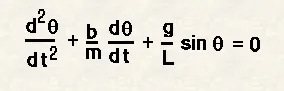
  ode solver function.
• For simulation the second order equation of the simple pendulum is:
• 
  To create a plot between angular velocity and displacement of simple pendulum by using ode45.

OBJECTIVE:

• The pendulum moves depends on the Newtons second law. When this law is written down, we get a second order Ordinary Differential Equation that describes the position of the "ball" w.r.t time.
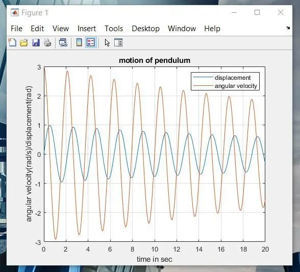
• Simulate the motion between 0-20 sec, for angular displacement=0,angular velocity=3 rad/sec at time t=0.
• By Using this information, animate the motion of the pendulum.

SOLUTION:

In the above equation,

g = gravity in m/s2,

L = length of the pendulum in m,

m = mass of the ball in kg,

b=damping coefficient.

parameters used are:

L=1 metre,

m=1 kg,

b=0.05.

g=9.81 m/s2.

THEORY :

A second order ordinary differential equation is an ordinary differential equation in which any derivatives with respect to the independent variable have order no greater than 2.

Ordinary differential equations helps us to solve the many engineering systems. Such as harmonic motions, vibrarions, damping,etc.

For designing a simple pendulum it consists of a mass ‘m’ hanging from a string of length ‘l’ and fixed at a pivot point . When displaced to an initial angle ’θ’ and released, the pendulum will swing back and forth with periodic motion.

This ODE represents the equation of motion of a simple pendulum with damping in the below equation

GOVERNING EQUATIONS :
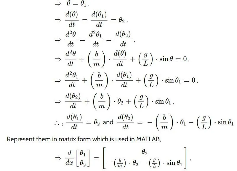
To solve the above equation in MATLAB, we need to transform the given second order ODE into first
order ODE as

MATLAB CODE:

clear all
close all
clc

%inputs
b=0.05;
l=1;
g=9.81;
m=1;

%inital condtion
theta_0=[0;3];

%time points
t_span=linspace(0,20,300);

%solve ode
[t,results]= ode45(@(t,theta) ode_func(t, theta,b,g,l,m),t_span,theta_0);
plot(t, results(:,1))
hold on
plot(t,results(:,2))
legend('displacement','angular velocity')


%Animating the transient motion of thesimple pendulum
figure(2)
ct=1;
for i=1:length(results(:,1))
 x0=0;
 y0=0;

 x1=l*sin(results(i,1));
 y1=-l*cos(results(i,1));


 plot([0 0],[-1.5 0.5])
 hold on
 plot([x0 x1],[y0 y1],'linewidth',1,'color','b')
 axis([-1.5 1.5 -1.5 0.5])
 plot(x1, y1,'o','MarkerSize',20,'color','r')
 pause(0.0001)
 M(ct)=getframe(gcf)
 hold off
 ct=ct+1

end
%making the video file
movie(M)
videofile=VideoWriter('simple_pendulum.avi','uncompressed AVI')
open(videofile)
writeVideo(videofile,M)
close(videofile)

ODE FUNCTION:

%FUNCTION CODE FOR SOLVING THE ODE:
function [dtheta_dt]= ode_func(t,theta,b,g,l,m)
theta1=theta(1)
theta2=theta(2)
dtheta1_dt=theta2;
dtheta2_dt= -(b/m)*theta2 - (g/l)*sin(theta1);
dtheta_dt=[dtheta1_dt;dtheta2_dt];
end

RESULTS:

GRAPH OF ANGULAR VELOCITY AND ANGULAR DISPLACEMENT FOR A RANGE OF 20 SEC:

animation of simple pendulum: https://youtu.be/MmarHtPHNSU

CONCLUSION:

• We have animated the simple pendulum using the ode45 solver where the second order is
  reduced to a simple differential equation where it is easy to solve the given equation.
• The animation is made using the different points of the bob and the motion of the simple
  pendulum is created