Week 1- Mixing Tee

Mixing Tee Joint

Pattan Akram

Aim: In this report airflow simulations of two different versions of mixing tee are studied namely short tee and long tee. The effects of the length and change in the mass flow rate on the outlet air temperature are studied.

Introduction:

Mixing tee joints are flow-controlled devices where the mixing of two different fluids is performed. It has two inlets and one outlet which are at 90 degrees. These are mainly used in nuclear plants and air-conditioning units etc.

Here is one inlet hot air is passed and the other with cold air. The standard deviation of the temperature is computed at the outlet of the pipe in order to measure the degree of variation in the temperature. Velocity and temperature are also measured. Different mesh size effects are also examined. Two different turbulent models k-epsilon, k-omega SST are used on the short tee model, and based on the results most suitable model is used for further use.

Here two different cases are examined:

Hot inlet temperature: C

Cold inlet temperature: C

Case-1: Case-2:

Short mixing tee with hot inlet velocity 3m/sec long mixing tee with hot inlet velocity 3m/sec

Momentum ratio: 2, 4 Momentum ratio: 2, 4

Momentum ratio = velocity at cold inlet / velocity at hot inlet.

Case 1:

Case 1 has two subcases with differing with two momentum ratios which yields Case1A & Case1B

Case 1A:

Momentum ratio: 2

Hot air inlet velocity: 3 m/sec

Cold air inlet velocity: 6m/sec

Pre-processing/Space claim:

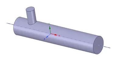
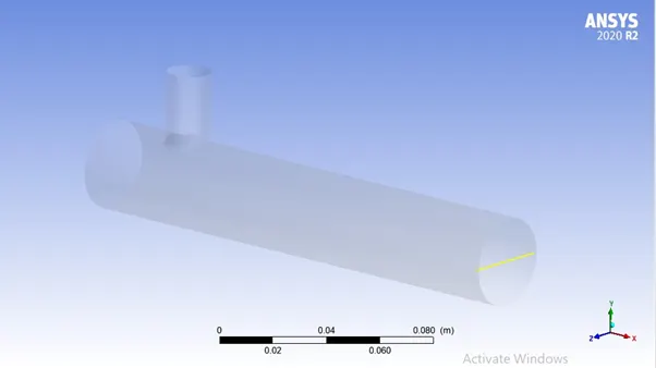
The CAD model is imported and the wet volume of the tube is extracted.

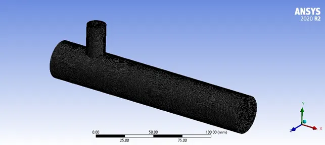
Mesh: The names of the boundary are applied and the meshing is done. Mesh metrics is also observed in order to check the quality of the mesh.

Element Size: 0.5mm

No of nodes: 3152

Elements: 14330

Type of mesh: Tetrahedral

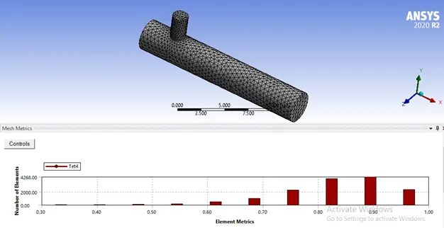
In the above image, we can see that the maximum number of elements are present in 90% quality, and also we have few elements in the least quality between 30%-40%

Setup:

In order to select the best suitable turbulent model for future analysis, we examine both the k-epsilon and k- omega. In the following manner.

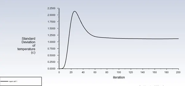
Area weighted averaged of velocity & temperature, Standard deviation of temperature at exit using k-epsilon model CASE 1A:

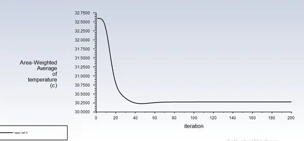
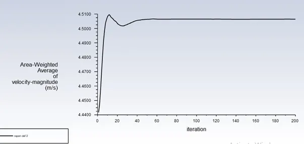
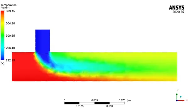
Here the contour plots of the velocity and the temperature are created on the XY-plane of the model k-epsilon

Temperature contour Plot:

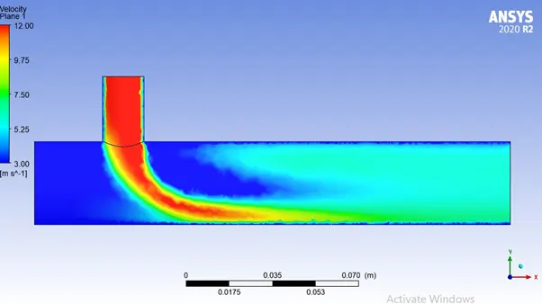
Velocity Contour Plot:

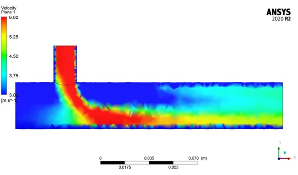
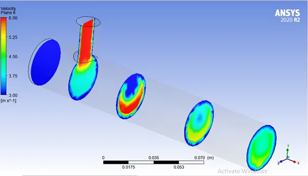
The above velocity contour is not good and it is due to the depletion in fine-ness of the mesh. Another study is carried as follows in order to show the effect of the fineness of the mesh in the contour.

Temperature contour across the pipe:

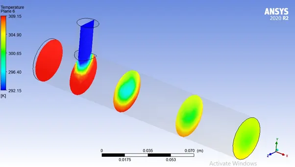
Velocity contour across the pipe:

Line Plots across the pipe: k-epsilon model

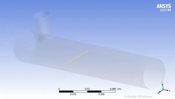
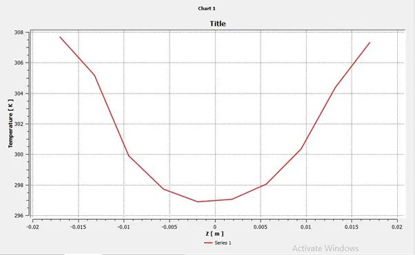
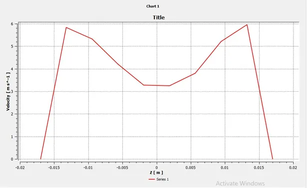
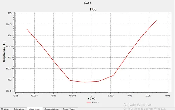
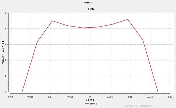
Line plots are created at two different locations one at the origin and the other at the exit and temperature and velocity lines are plotted on the z-axis by creating two lines at two different locations.

Line plots at line 1:

Temperature plot at line 1:

Velocity plot at line1:

Plots at line 2:

Temperature plot at line 2:

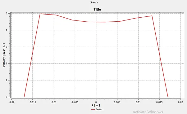
Velocity plot at line2:

K-OMEGA MODEL of Case-1A:

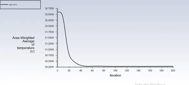
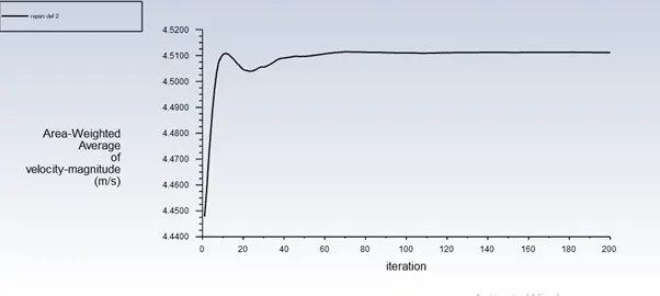
Line plots of Area weighted averaged of velocity & temperature, Standard deviation of temperature at exit using k-omega SST model CASE 1A:

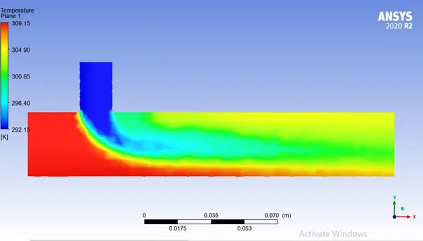
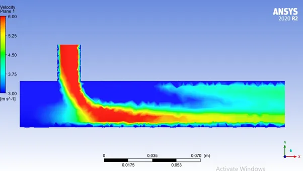
Temperature and velocity contour plots of Case 1A using k-omega model:

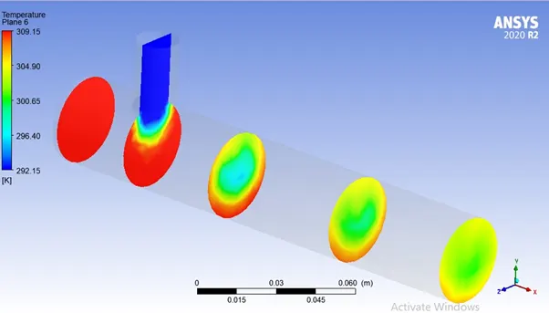
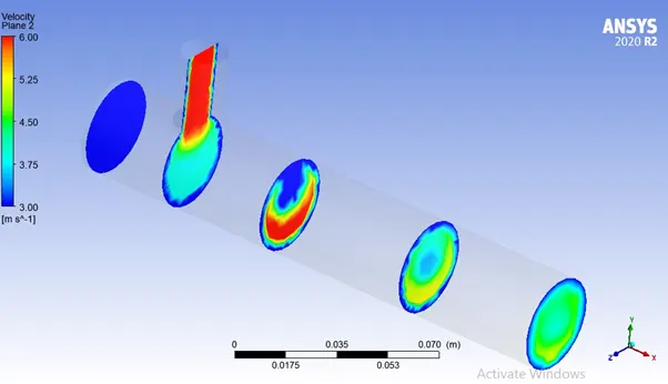
Temperature and velocity contour across the pipe:

Line Plots across the pipe: k-omega model

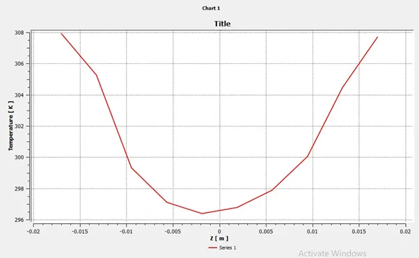
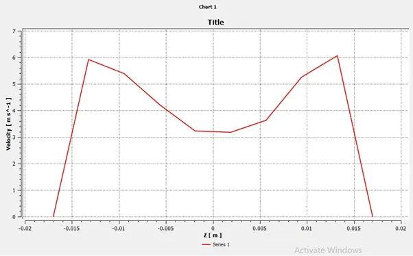
Line plots are created across the pipe in the previously used locations.

Temperature plot at line 1:

Velocity plot at line1:

Temperature plot at line 2:

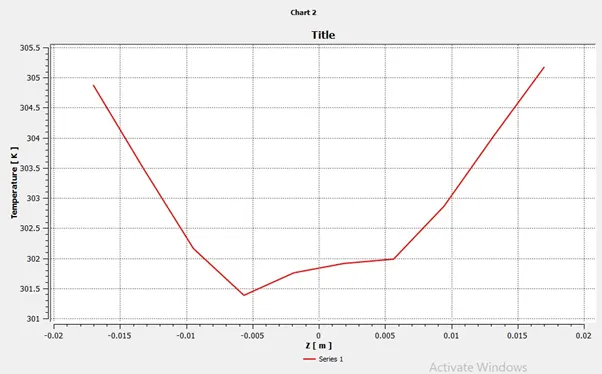
Velocity plot at line2:

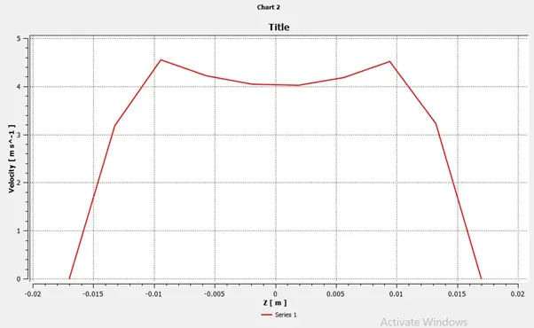
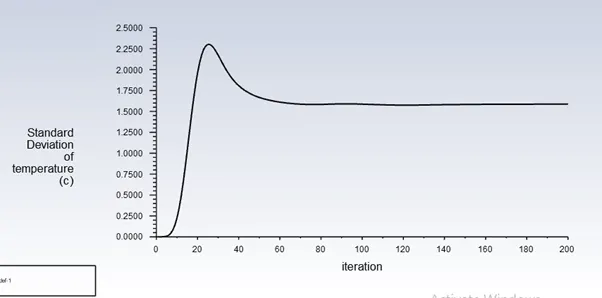
By looking at the standard deviation graph of the turbulent model k-epsilon and the k-omega. We can observe that the standard deviation of the temperature using the k-epsilon model is much less than the k-omega where it goes to steady-state at a value of approximately 1.59 and in the other case i.e in k epsilon model the system goes to steady-state at a value of 1.25.

The remaining two line plots of the area-weighted average of the temperature and the velocity at the exit are the same for both the k-omega and k-epsilon models.

We can also observe that from the line plots across the pipe at the exit the temperature in the direction of z-direction is uniform for a k-epsilon model whereas in k-omega it is not uniform and therefore resulting in the leek of high temperature at some of the points due to the lack of proper mixing.

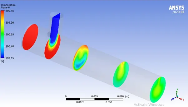
When we observe the contour plots k-epsilon model has a fine mixing than the k-omega model which results in the lower exit temperature of the k-epsilon than the other.

Since lesser standard deviation results in the better effectiveness of the mixing, we choose the k-epsilon model for future analysis.

Case 1A with lesser Mesh Size: 2mm

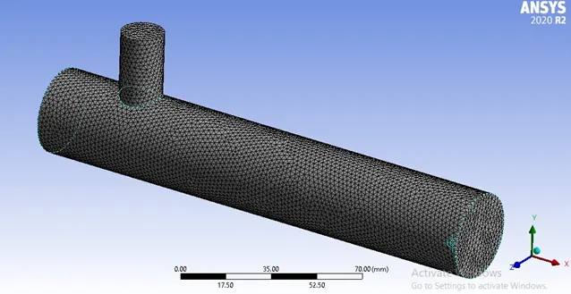
The above picture shows the mesh of the body with a mesh size 2mm.

No of nodes: 2137

Elements: 105865

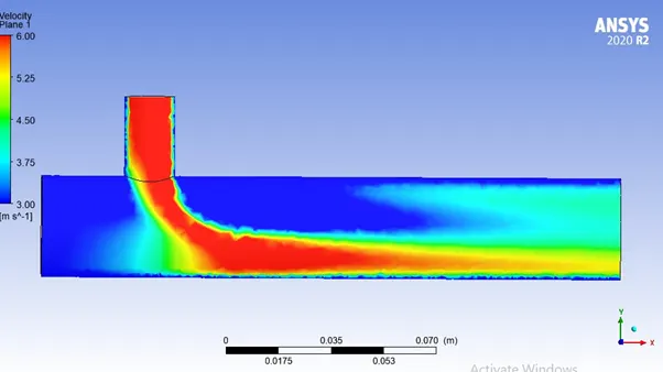
The following are the contour results

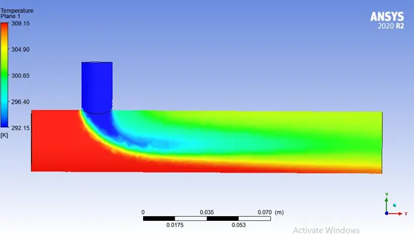
Case 1A with lesser Mesh Size: 1mm

The following are the contour results

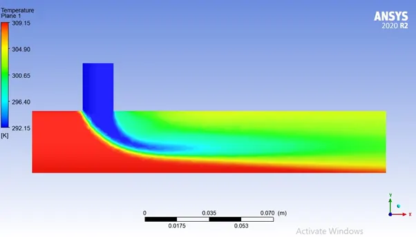
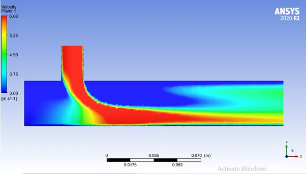
By watching the above contour plots we can see that the finer the mesh finer and smoother will be the results and we can expect the results are also fine.

Case 1B:

Momentum ratio: 4

Hot air inlet velocity: 3 m/sec

Cold air inlet velocity: 12m/sec

Element Size: 2mm

No of nodes: 2137

Elements: 105865

Type of mesh: Tetrahedral

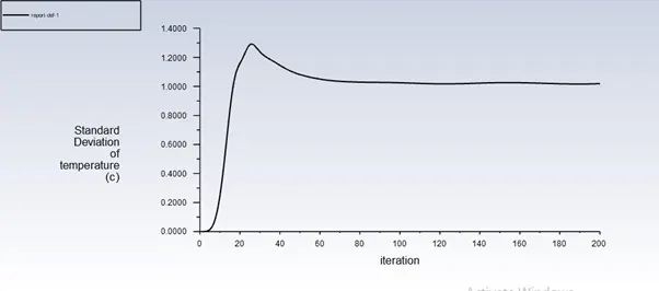
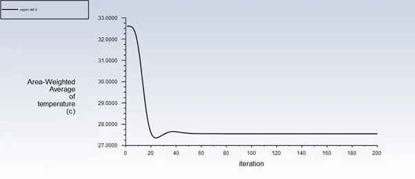
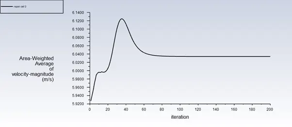
The following are the line plots of the area-weighted average temperature and area-weighted average velocity and standard deviation of the temperature at the exit.

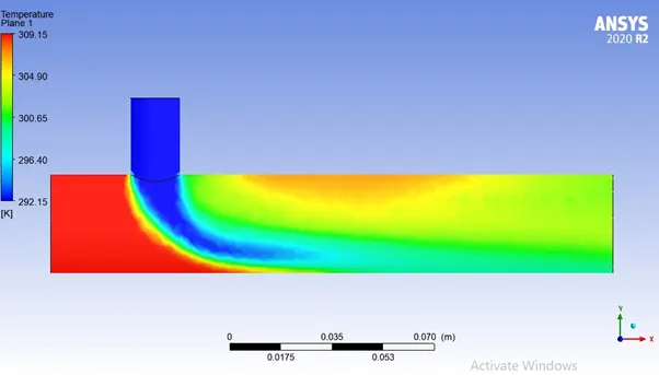
The following are the velocity and temperature contours:

Temperature contour across the pipe:

Velocity contour across the pipe:

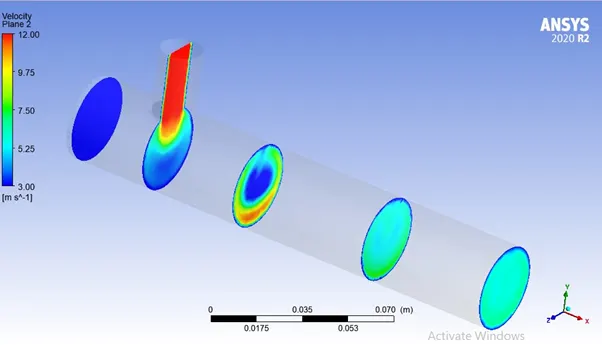
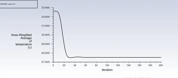
From the above graphs, we can see that the case with the highest cold air velocity has less standard deviation which gives the best effectiveness of mixing. Hence in the case of the long tee joint, we will study the case with the highest cold air velocity.

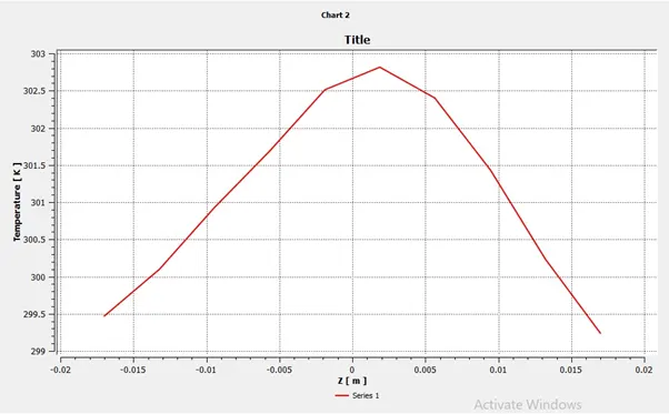
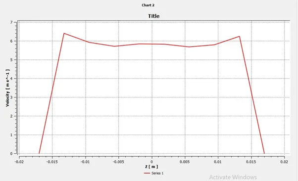
Line Plots across the pipe:

Plot at line 1:

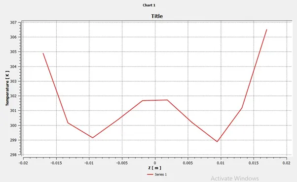
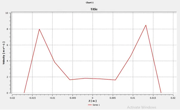
Plot at line 2:

Case 2B:

Momentum ratio: 4

Hot air inlet velocity: 3 m/sec

Cold air inlet velocity: 12m/sec

Following are the line plots of the area-weighted average of temperature, velocity, and standard deviation of the temperature at the exit.

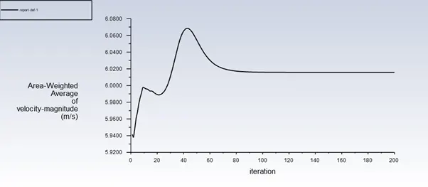
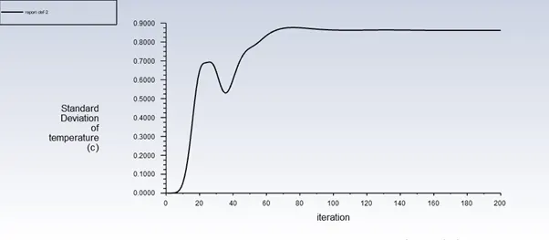
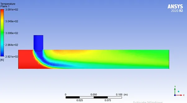
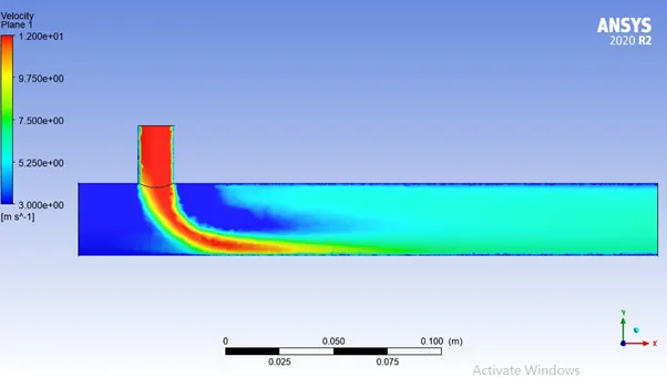
The following are the contour plots of the velocity and temperature:

Contour plots across the pipe:

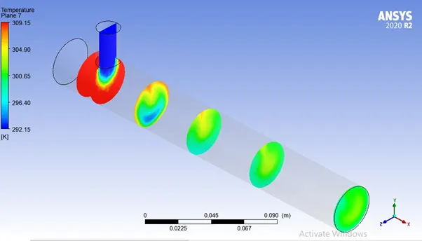
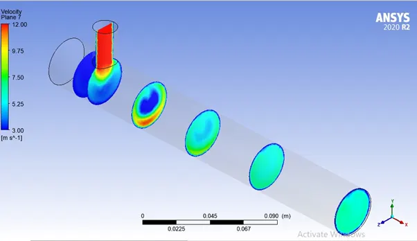
Line plots of temperature and velocity across the pipe:

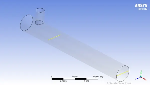
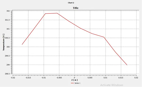
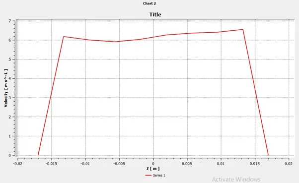
In the above picture, we can see that two lines are created one at the origin and the other at the outlet in order to draft temperature and velocity plots along those lines.

Temperature and velocity plots along Line 1:

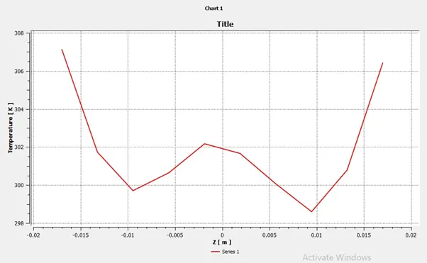
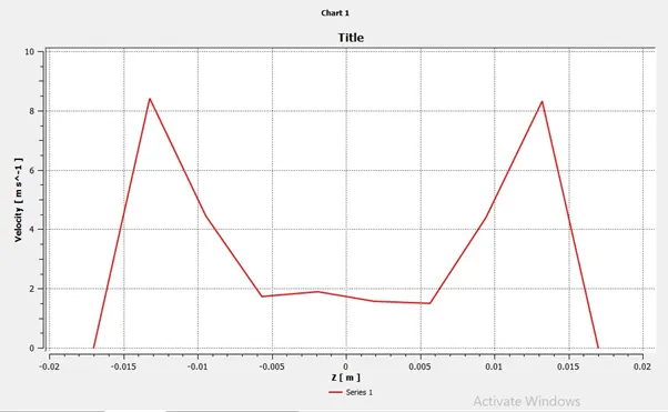
Temperature and velocity plots along line 2:

Case 2A:

Momentum ratio: 3

Hot air inlet velocity: 3 m/sec

Cold air inlet velocity: 06m/sec

Mesh size: 2mm

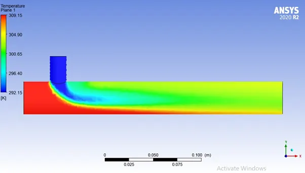
Contour plots of temperature and velocity:

Line plots:

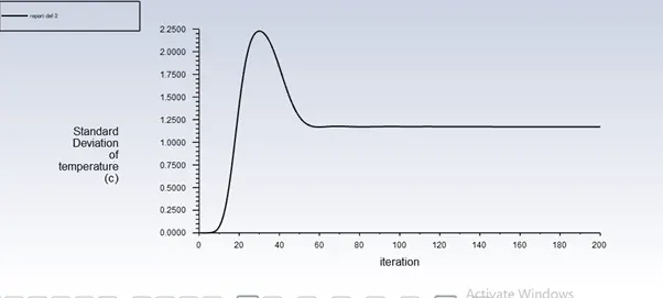
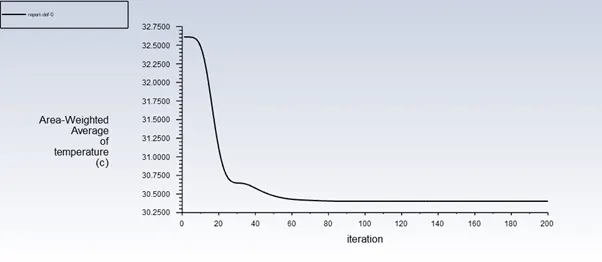
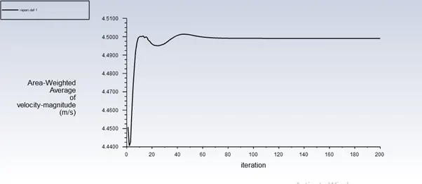
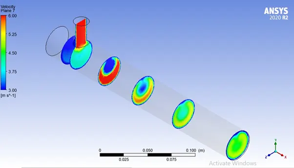
Temperature and velocity contour across the pipe:

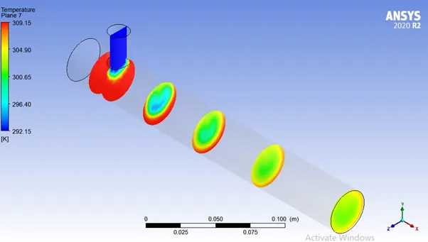
Line plot across the line 1&2:

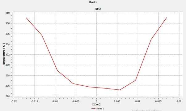
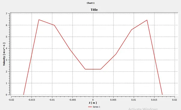
Temperature and velocity plots along line 1:

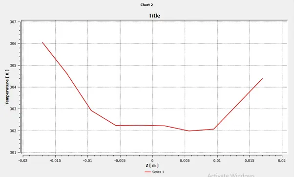
Temperature and velocity plots along line 2:

Conclusion:

• In case of 1A, the exit temperature is a little higher than Case 1B mainly due to improper mixing of the air as in case 1A the cold air inlet velocity is lower than the case 1B.
• When we compare the short tee with the long tee in the case of high cold air velocity we can see that the standard deviation of the temperature at the outlet is lower in the long tee than the short tee which is proof of good mixing.
• From the above analysis, we can see that a long tee with high inlet cold air is best when compared to the other configurations.
• Since K-epsilon predicts well far from the boundaries whereas k-omega is best suited for the near the wall-flow region. In this scenario, as we are interested in the outlet temperature and proper mixing k-epsilon model is well suitable.