Week 1 : Exploring the GUI of GT-POWER

Aim:Exploring the GUI of GT-POWER

objective:

1. Explore the GUI of GT SUITE and list down modules available with brief description.

2. Locate following settings:

   • Time control flag
   • Time step and solution control
   • Integrator/Solver type

3. Explore intercooler tutorial and note down all settings of:

   • Run setup
   • Advanced setup
   • Plot setup
   • Output setup
4. Problem

Given

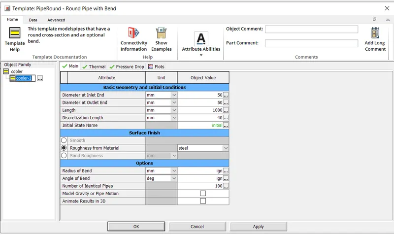
• Diameter of cooler inlet and outlet pipe= 50 mm
• Length of the CAC= 1000 mm
• Inlet mass flow rate = 1200 kg/ h at 100 degC
• Outlet pressure 2 bar at 30 deg C

• Calculate the Average heat transfer at Charge air cooler (CAC)
• Calculate pressure drop across CAC

theory:

GT Suite is a software suite for engineering and simulation of complex systems, such as vehicles, powertrains, and aerospace systems. It is used by engineers and researchers to model and simulate the behavior of these systems and predict their performance under various conditions. The suite includes several modules, each designed for specific types of analysis and simulation. Some of the modules available in GT Suite include:

1. GT-Power: A tool for the modeling and simulation of internal combustion engines and powertrains.

2. GT-Drive: A tool for the modeling and simulation of electric and hybrid vehicles.

3. GT-Suite Vehicle Dynamics: A tool for the modeling and simulation of vehicle dynamics, including suspension, steering, and braking systems.

4. GT-Suite Transmission: A tool for the modeling and simulation of transmission systems, including manual and automatic transmissions.

5. GT-Suite Thermal: A tool for the modeling and simulation of thermal systems, including cooling and heating systems, and HVAC systems.

6. GT-Suite Fluid Dynamics: A tool for the modeling and simulation of fluid dynamics, including fluid flow, heat transfer, and combustion processes.

7. GT-Suite Control: A tool for the modeling and simulation of control systems, including engine and powertrain control systems.

8. GT-Suite Model Library: A library of pre-built models for various types of systems, including engines, powertrains, and vehicles, that can be used as starting points for building new models.

9. GT-Suite Optimization: A tool that allows to optimize the design of systems using various optimization methodologies.

These are some of the modules of GT Suite, but the list may change as new updates come out or new modules are added.

Time Control Flag: Defines the global simulation type with regard to time. One of the following options:

• periodic indicates that the model contains at least one circuit which contains a periodic event (i.e. engine cylinder “cycle”) and therefore requires tracking of results with respect to angle over each cycle. Any model that includes an ' EngineCrankTrain', ' CrankAnalysis' , or ' EngineCrankShaft' part should use the periodic option. Note that the simulation duration for a periodic simulation can be specified in cycles or in time, whichever is most convenient.

• continuous indicates that the simulation includes no periodic event, and therefore has no need to track results with respect to a cyclic angle. This is the typical setting for models that contain only quasi-steady fluid circuits such as coolant or underhood air. The simulation duration for a continuous simulation is typically specified in time.

to open time contol flag open run setup

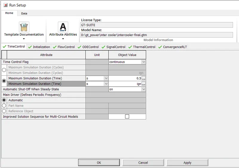
time control flag setup

Time Step and Solution Control Object:

Name of the ' FlowControlExplicit', ' FlowControlImplicit', or ' FlowControlQS' reference object that can be used to define the numerical parameters for the explicit, implicit, or quasi-steady flow solver, respectively.

FlowControlExplicit:This reference object defines numerical and other solver settings (real gas, flow loss models, and friction and heat transfer) for the explicit flow solver.

FlowControlImplicit:This reference object defines numerical and other solver settings (real gas, flow loss models, and friction and heat transfer) for the implicit flow solver.

FlowControlQS: This reference object defines numerical and other solver settings (real gas, flow loss models, and friction and heat transfer) for the quasi-steady flow solver.

It is used in the Time Step and Solution Control Object attribute in the Setup > Run Setup > FlowControl folder.

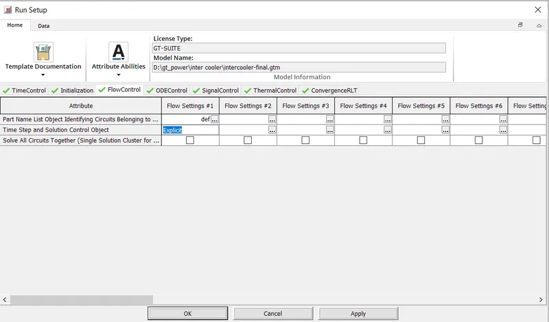
flow control

Integrator/Solver type:

Integrator/solver type used in the time-marching of all ODEs including mechanical, electrical and magnetic libraries. For recommendations based on the application, please see the color-coded table immediately following this text.

•Explicit-Adams-PECE Explicit Adams-Bashforth-Moulton predictor-corrector integration scheme with variable order accuracy. This integrator is recommended for large non-stiff problems, problems with a high maximum time step which have different scales and real time applications. It requires a tuning process in order to optimize its functionality, please contact Email: [email protected] for more details.

•Explicit-Runge-Kutta Explicit Runge-Kutta integration scheme that is 5 th order accurate. This integrator is recommended for non-stiff problems.

•Implicit-Trapezoidal Implicit Trapezoidal integration scheme that is 2 nd order accurate. This integrator is recommended for moderately stiff problems.

•Implicit-H.H.T. Implicit Hilber-Hughes-Taylor integration scheme that is 2 nd order accurate. This integrator is recommended for moderately stiff problems.

• Implicit-Radau2 Implicit 2-stage Radau integration scheme that is 3 rd order accurate. This integrator is recommended for stiff problems.

• Implicit-Radau3 Implicit 3-stage Radau integration scheme that is 5 th order accurate. This integrator is recommended for stiff problems.

•Implicit-S.D.C.3 Implicit 3-stage Spectral Deferred Correction (S.D.C.) integration scheme that is 5 th order accurate. This integrator is recommended for very stiff problems.

The following options are for very specific use cases:

•Static-Solver Static equilibrium of a mechanical system/circuit will be performed. This is ONLY for flexible/rigid primitive systems with zero degrees of freedom. All degrees of freedom must be removed with constraints (RevoluteJoint, Constraint2D, etc.) or reacted by Spring* objects.

•Explicit-Euler Explicit Euler integration scheme that is 2nd order accurate. This integrator may be used for very simple non-stiff systems where CPU time is critical. Medium and high-frequency results may differ significantly from other integrators.

A system is considered to be stiff when there are vastly different oscillation timescales. In other words, very high and very low frequencies combined in the same model. Implicit integrators require more CPU time per individual timestep, but this is outweighed by the ability to take larger steps for stiff systems.

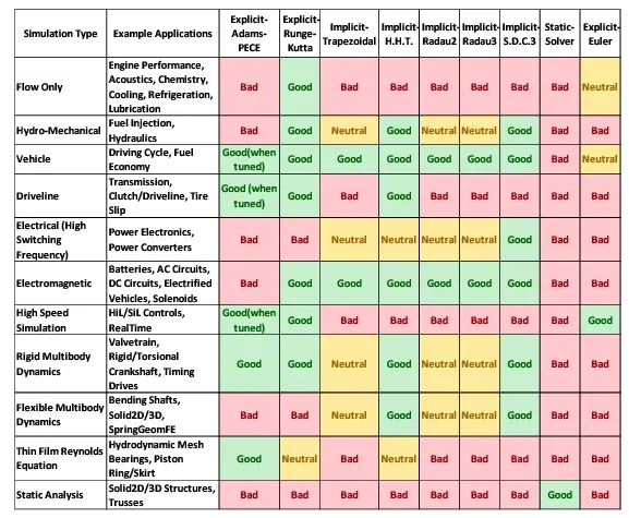
ode solver for different type of simulation

It is used in the Time Step and Solution Control Object attribute in the Setup > Run Setup > ODEControl folder.

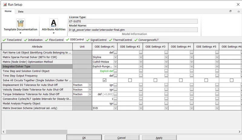
ODEControl

PROBLEM

open a new file

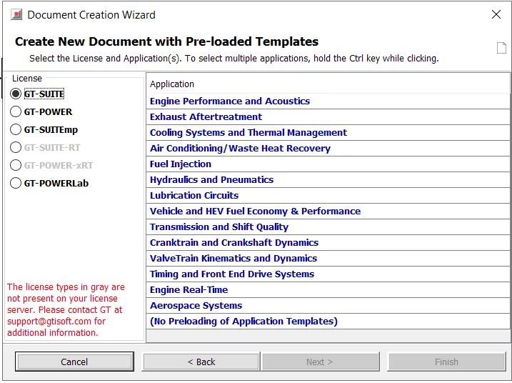
copy tutorial file

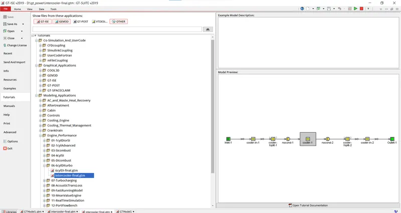
save that file in a different folder

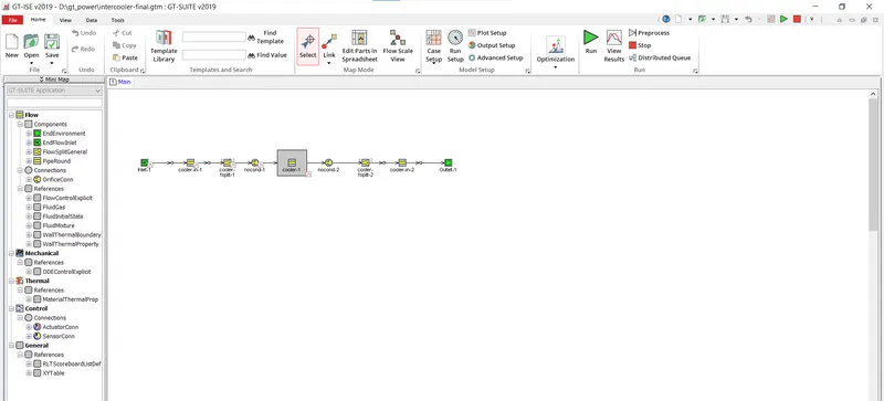
workspace

inlet setup

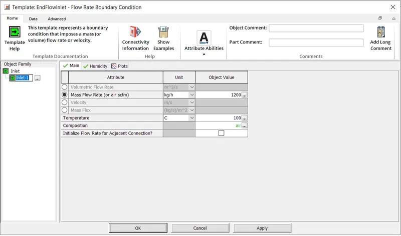
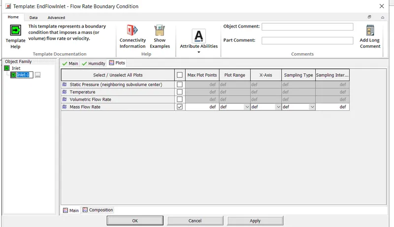
cooler in 1

do not chage in cooler in 1 and 2 just setup plots want to see result

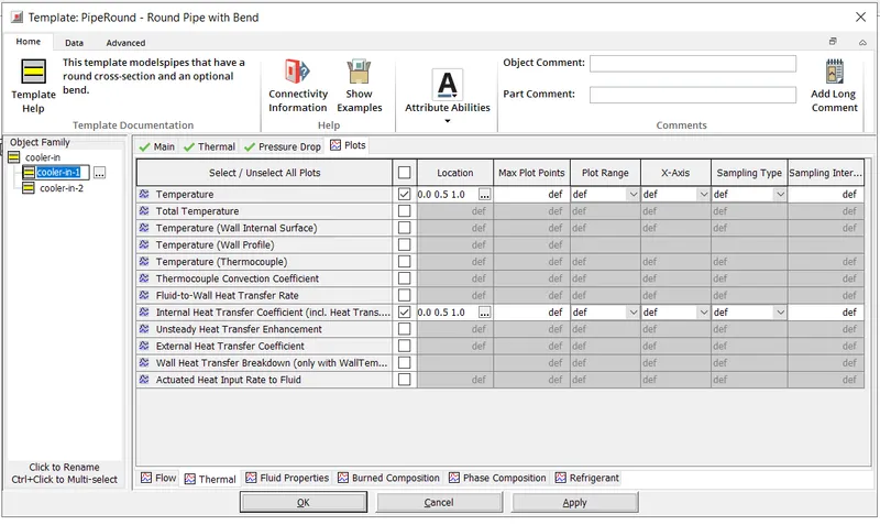
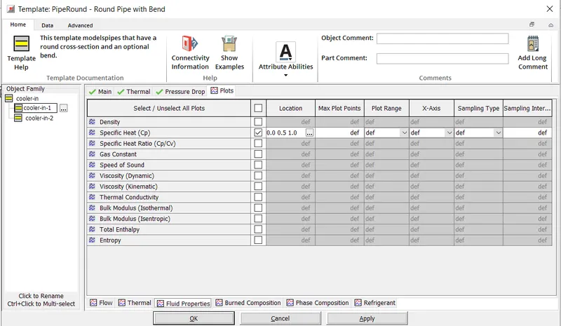
temprature and specific heat plot

in cooler-fsplit-1 and 2 do not chanegeany thing

OrificeConn no change in here also

cooler-1 change inlet dia and outlet dia and length of cooler

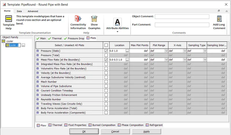
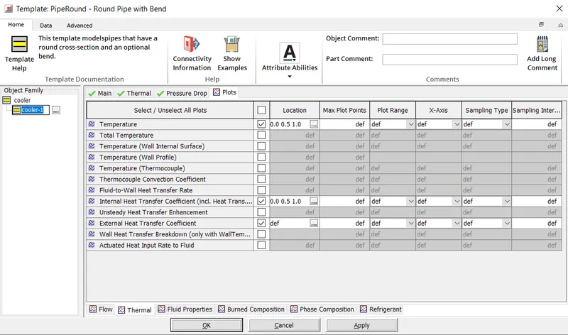
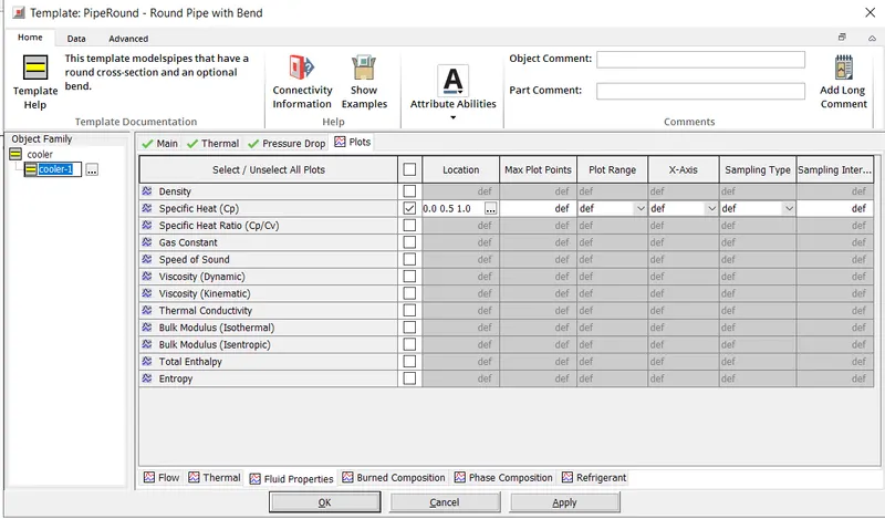
plots

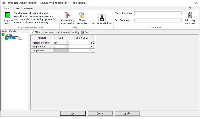
outlet setup

Run setup here run parameters were defined

just chage the simulation time and keep every thing as it is

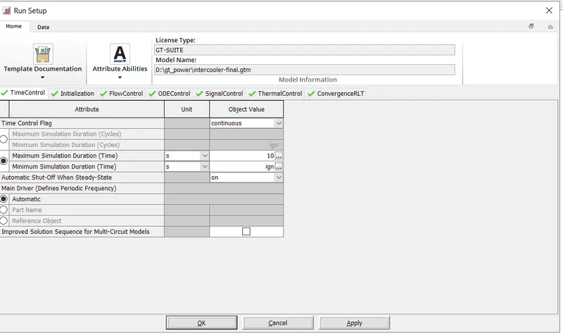
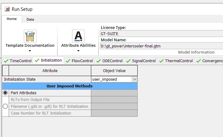
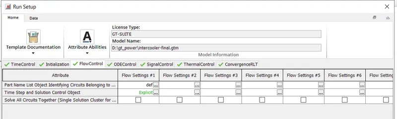
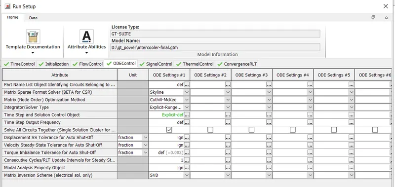
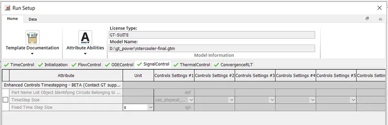
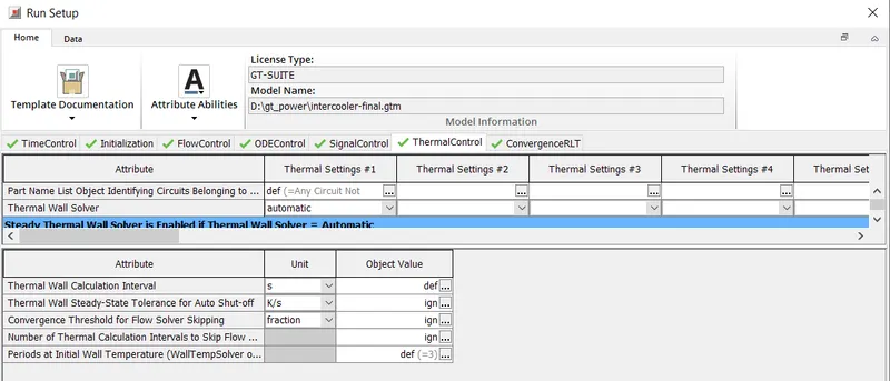
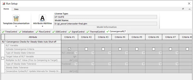
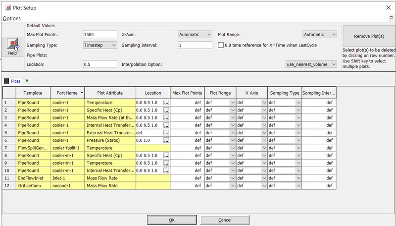
plot setup Cycle and/or time plots may be requested by selecting the appropriate plot from the "Plot Options" folder within each part. Each of these requests will result in a plot being stored.

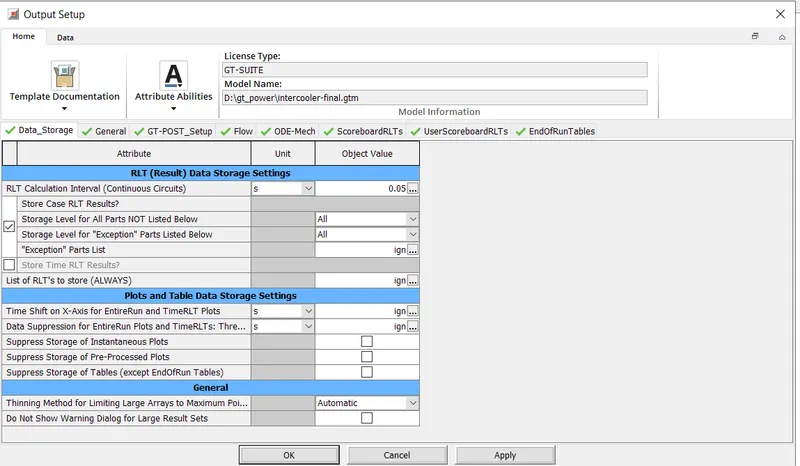
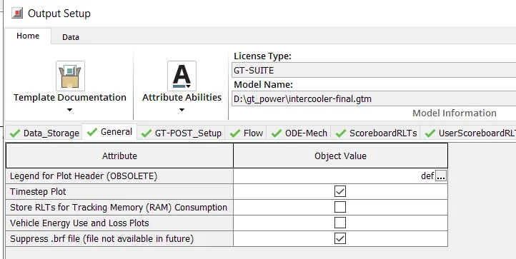
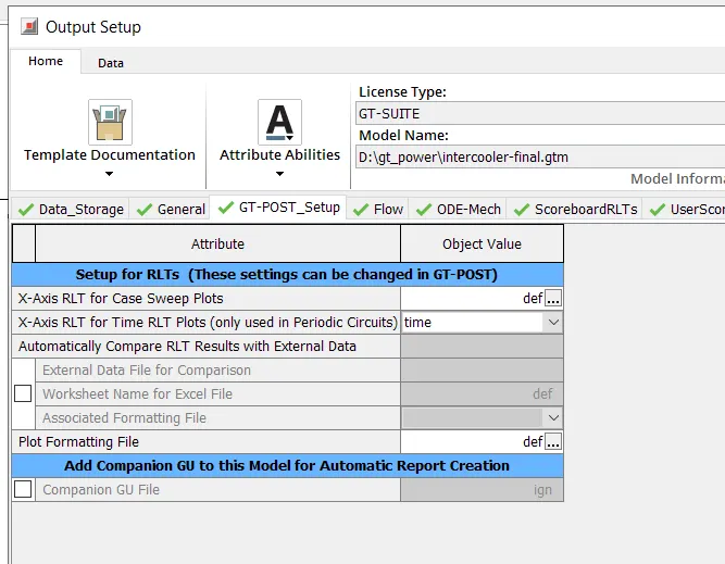
output setup here output file storage and saving setting were controled

do not chage anything in output setup

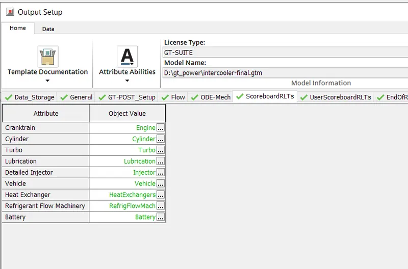
advance setup here no chages are made

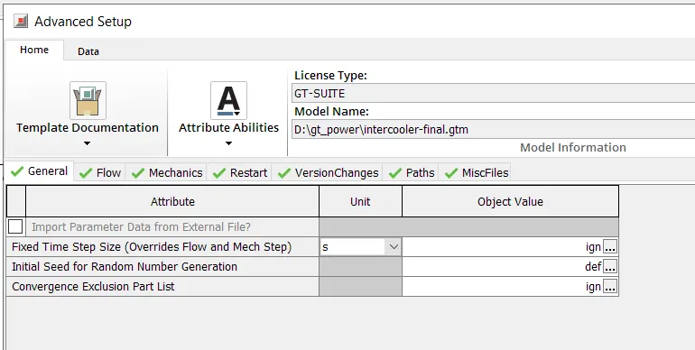
after this setup run the smulation

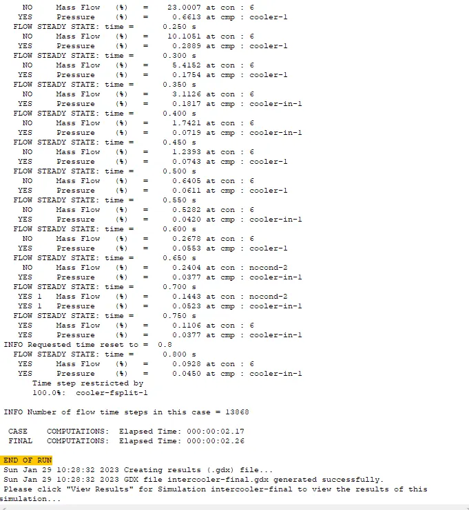
after simulation end

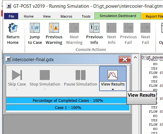
click on view results

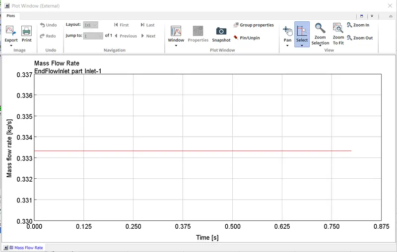
Results

mass flow rate at inlet

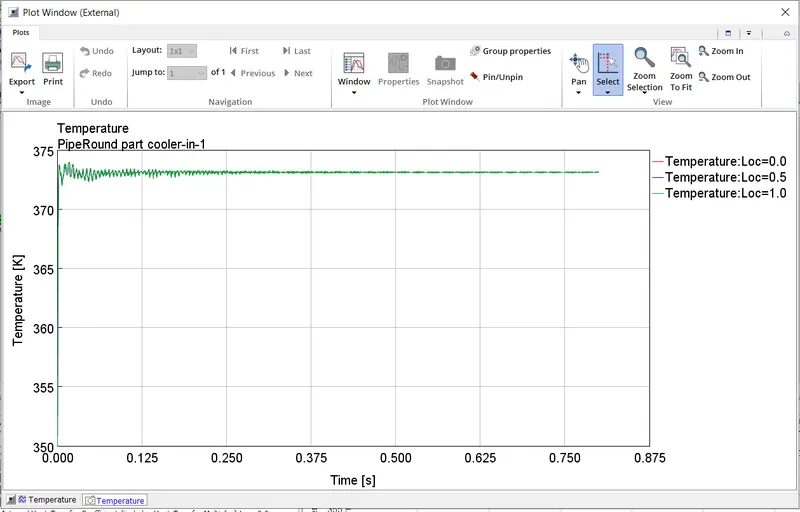
temprature in cooler in 1

results in cooler 1

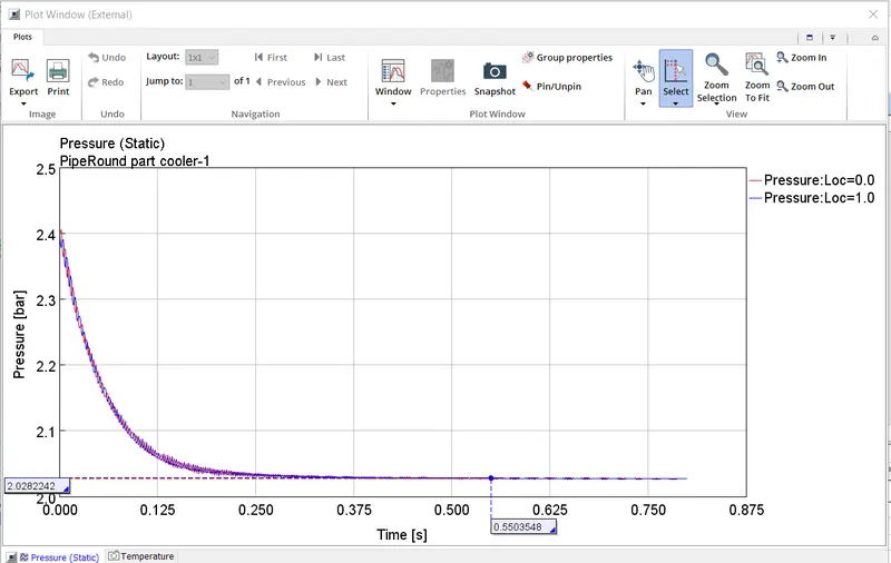
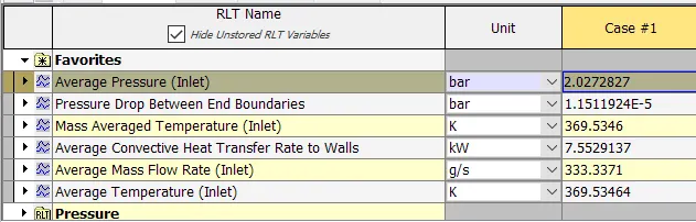
pressure at inlet and outlet

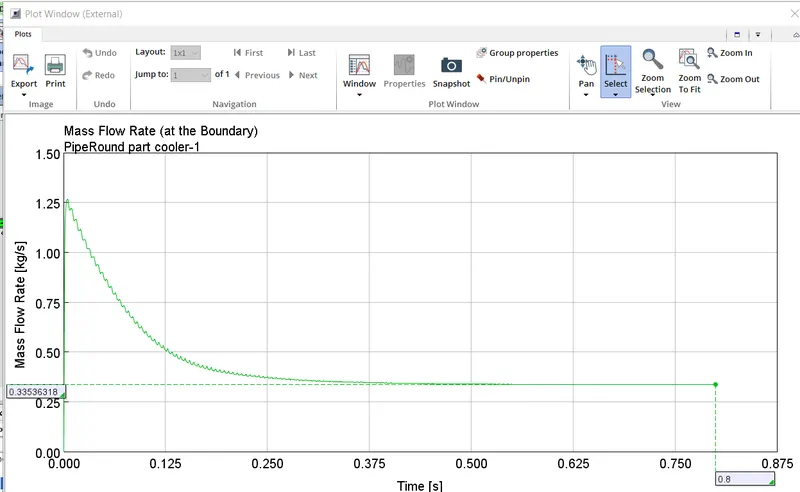
mass flow rate at inlet

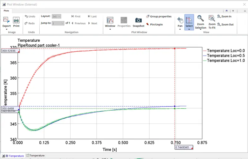
temprature at inlet,mid point and outlet

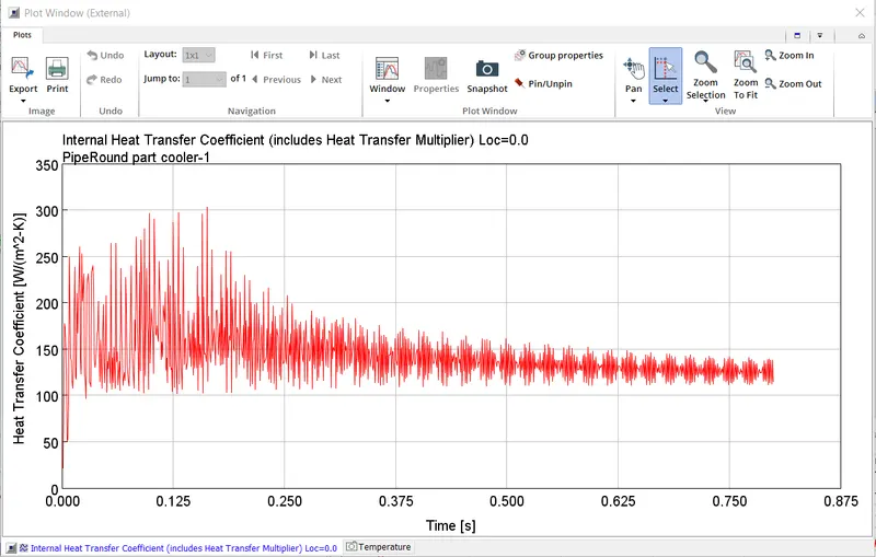
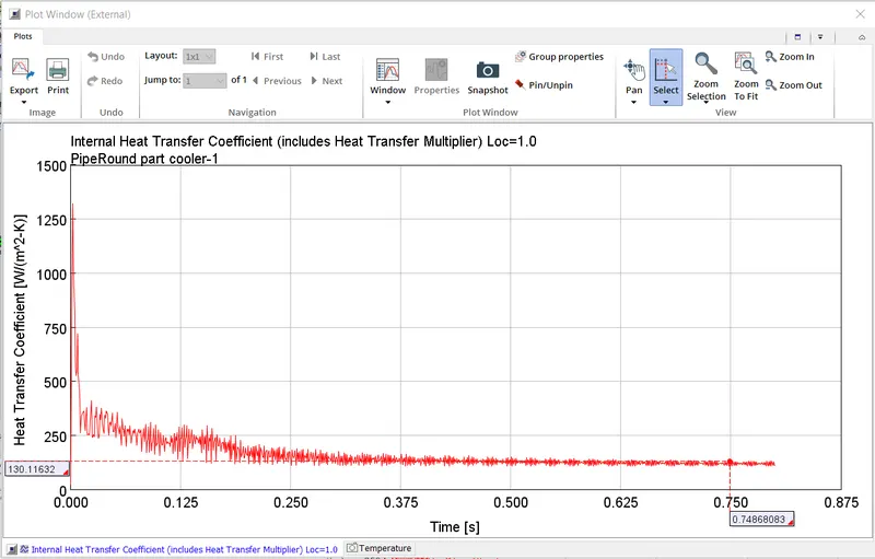
heat transfer coefficient at inlet and outlet

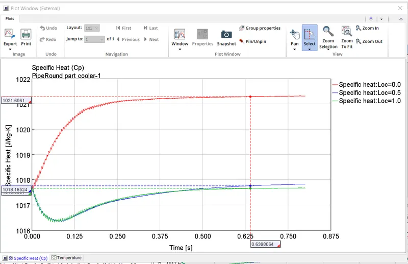
specific heat at inlet and outlet

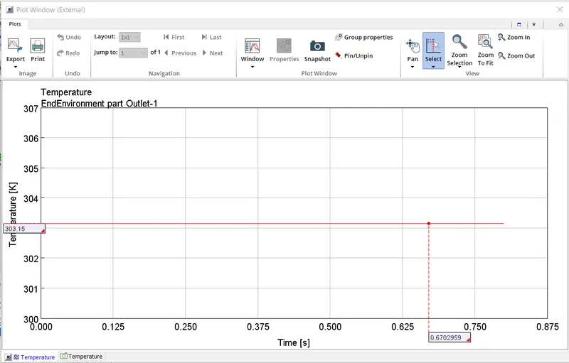
temprature at outlet of the cooler

conclusion

the set is done using tutorial file requied correction were made the simulation ran smoothly and the results were convencing

Average heat transfer at Charge air cooler (CAC):

`Q=m_f*c_p*(T_(i n)-T_(out))`

where

m_f is mass flow rate of fluid in m/s

c_p specific heat of fluid in j/kg-k

T_in temp at inlet

T_out temp at out

`Q=0.333*1020*(373-350)`

Q=6.793 kj

6.793 kj heat is removed from fluid

pressure drop across CAC

presssure drop across the boundaries is given