Week 1 : Exploring the GUI of GT-POWER
Exploring the GUI of GT Suite
Aim:
1. To explore the GUI of GT-Suite and understand the settings and available options, and to get accustomed to the software.
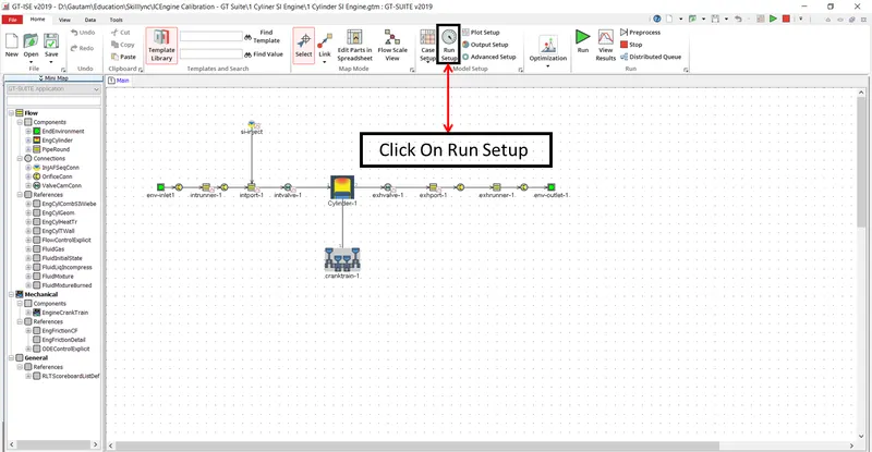
2. Locate the Settings (Time Control Flag, Time Step & Solution Control, Integrator/Solver Type).
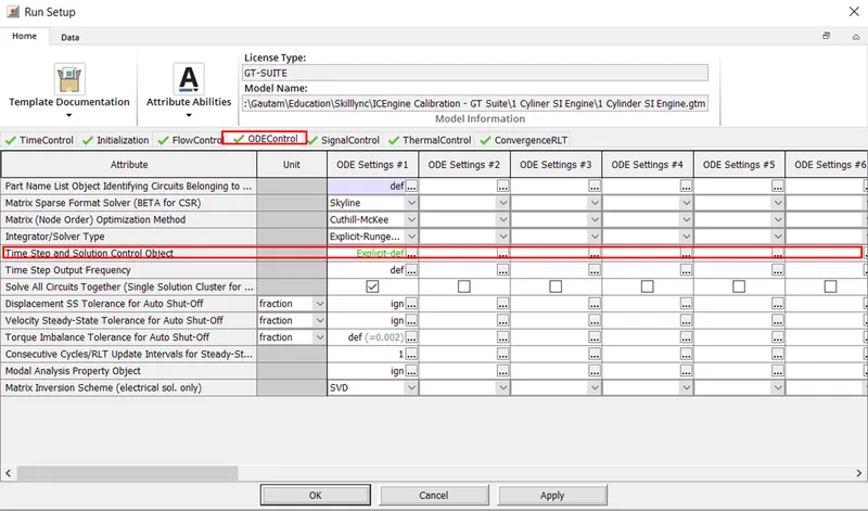
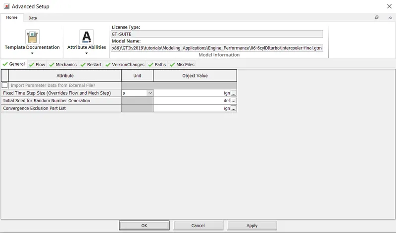
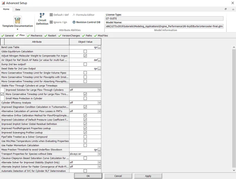
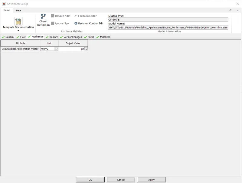
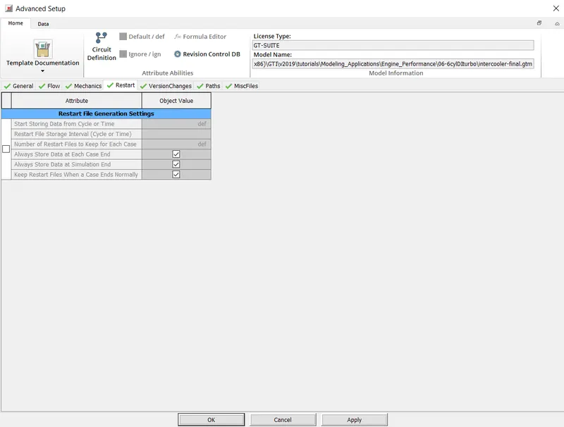
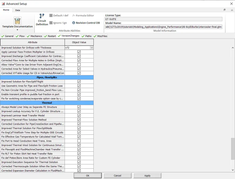
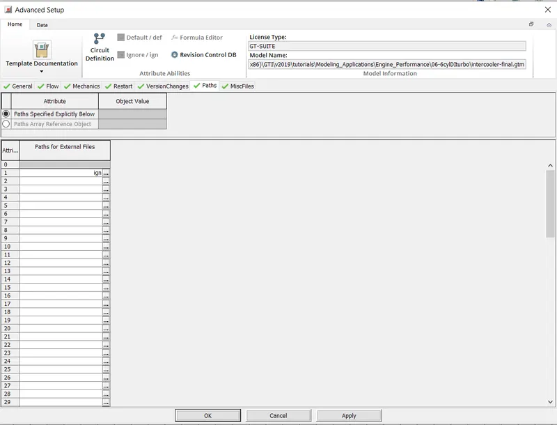
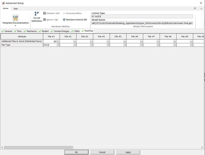
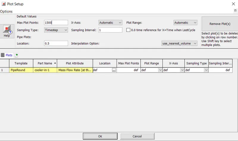
3. Explore intercooler tutorial (Run Setup, Advanced Setup, Plot Setup, Output Setup).
4. To simulate an Intercooler and to calculate the average heat transfer rate and pressure drop across the system.
1. GUI of GT-Suite:
GT-SUITE is the leading simulation tool with capabilities and libraries aimed at a wide variety of applications and industries. It offers engineers functionalities ranging from fast concept design to detailed system or sub-system/component analyses, design optimization, and root cause investigation.
GT Suite span across various industries, to know more about GT Suite click on the links given below:
By Industries:
By Application:
2. Locate the Settings:
- Time Control Flag:
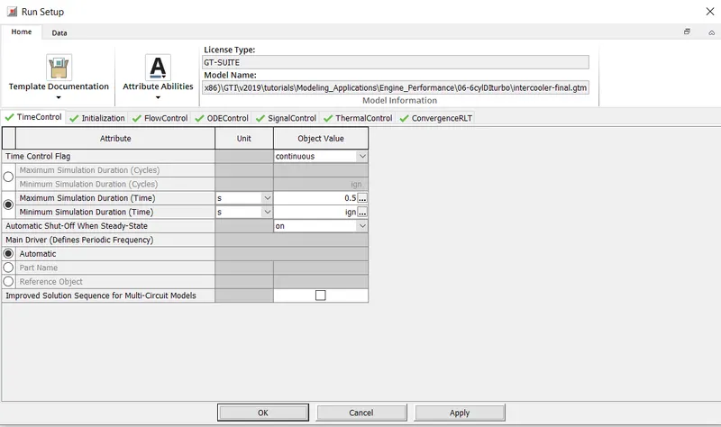
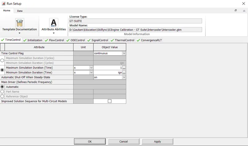
Time Control is used to define the simulation duration and time-controlling variables. The attributes in this folder must be defined for all simulations.
Types of Time Control Flag
Periodic: Indicates that the model contains at least one circuit which contains a periodic event (i.e. engine cylinder “cycle”) and therefore requires tracking of results with respect to angle over each cycle. Any model that includes an ' EngineCrankTrain', ' CrankAnalysis' , or ' EngineCrankShaft' part should use the periodic option. Note that the simulation duration for a periodic simulation can be specified in cycles or in time, whichever is most convenient.
Continuous: Indicates that the simulation includes no periodic event, and therefore has no need to track results with respect to a cyclic angle. This is the typical setting for models that contain only quasi-steady fluid circuits such as coolant or underhood air. The simulation duration for a continuous simulation is typically specified in time.
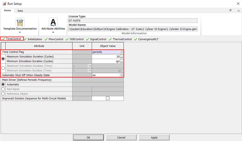
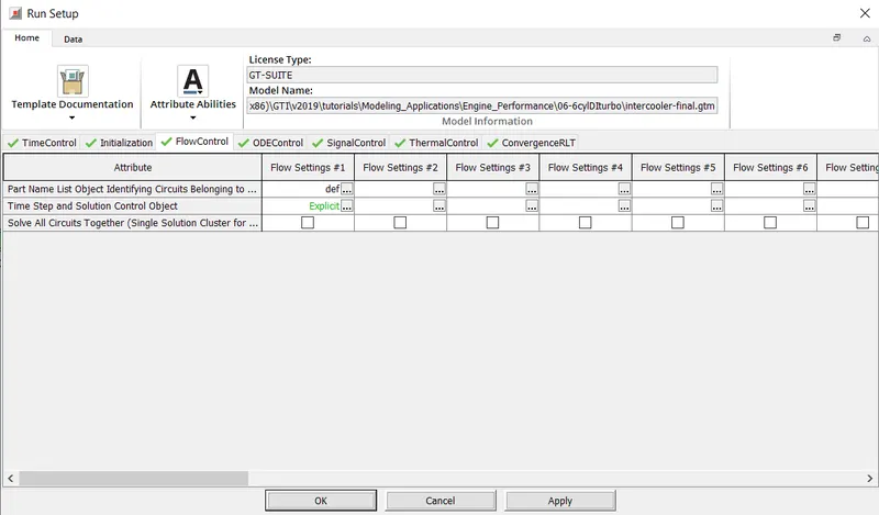
- Time Step and Solution Control:
Reference object that can be used to define the numerical parameters for the explicit, implicit, or quasi-steady flow solver, respectively
Flowcontrol Explicit: This object should be used when tracking high frequency wave dynamics is important. Typical examples include any analysis where crank angle resolved results are required, (engine performance, fuel injection, lubrication, etc.).
Flowcontrol Implicit: This object should be used for simulations where wave dynamics are not important (thermal warm-up, system behavior over long driving cycles, etc.). The implicit solver typically takes much larger time steps compared to the explicit solver. The implicit solver should only be used for simulations in which:
There are minimal wave dynamics in the system, or accurate prediction of wave dynamics is unimportant, AND, the maximum Mach number in the system is less than 0.3 (unless the attribute Compressible Flow Enhancement is turned "on").
For example, typically thermal management simulations (i.e. underhood/engine cooling, HVAC and Waste Heat Recovery) fall within this category, and using the implicit solver is recommended.
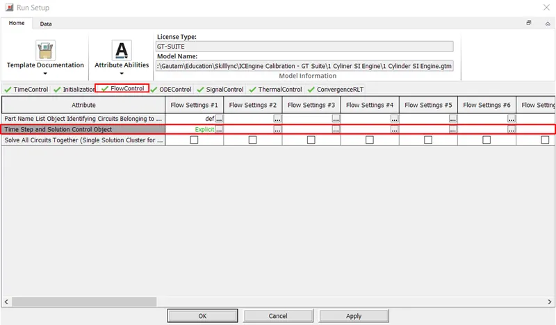
- Integrator/Solver Type:
Integrator/solver type used in the time-marching of all ODEs including mechanical, electrical and magnetic libraries. For recommendations based on the application, please see the color-coded table immediately following this text.
Explicit-Adams-PECE: Explicit Adams-Bashforth-Moulton predictor-corrector integration scheme with variable order accuracy. This integrator is recommended for large non-stiff problems, problems with a high maximum time step which have different scales and real time applications. It requires a tuning process in order to optimize its functionality, please contact Email: [email protected] for more details.
Explicit Runge-Kutta: integration scheme that is 5 th order accurate. This integrator is recommended for non-stiff problem
Implicit-Trapezoidal: Implicit Trapezoidal integration scheme that is 2 nd order accurate. This integrator is recommended for moderately stiff problems.
Implicit-H.H.T:Implicit Hilber-Hughes-Taylor integration scheme that is 2 nd order accurate. This integrator is recommended for moderately stiff problems.
Implicit-Radau2: Implicit 2-stage Radau integration scheme that is 3 rd order accurate. This integrator is recommended for stiff problems.
Implicit-Radau3: Implicit 3-stage Radau integration scheme that is 5 th order accurate. This integrator is recommended for stiff problems.
Implicit-S.D.C.3: Implicit 3-stage Spectral Deferred Correction (S.D.C.) integration scheme that is 5 th order accurate. This integrator is recommended for very stiff problems.
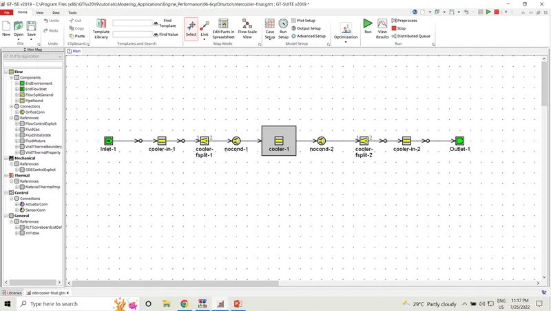
3.Explore Intercooler Tutorial:
- Run Setup:
Time Control
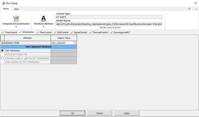
Initialization
Flow Control
ODE Control
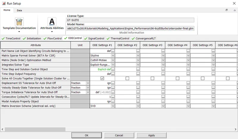
Signal Control
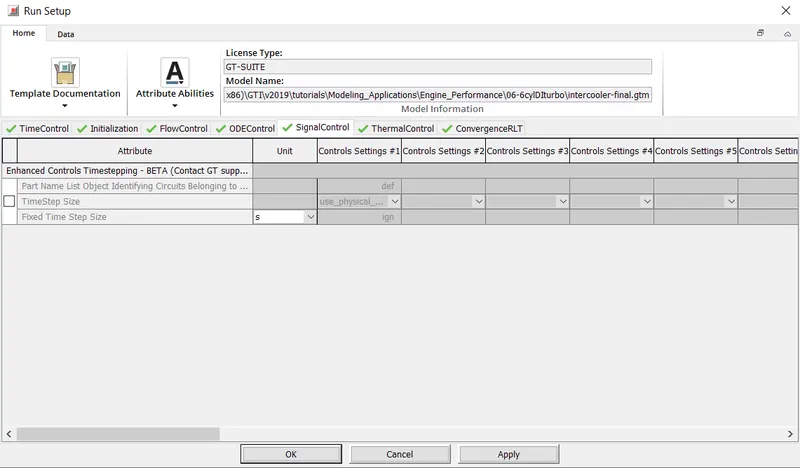
Thermal Control
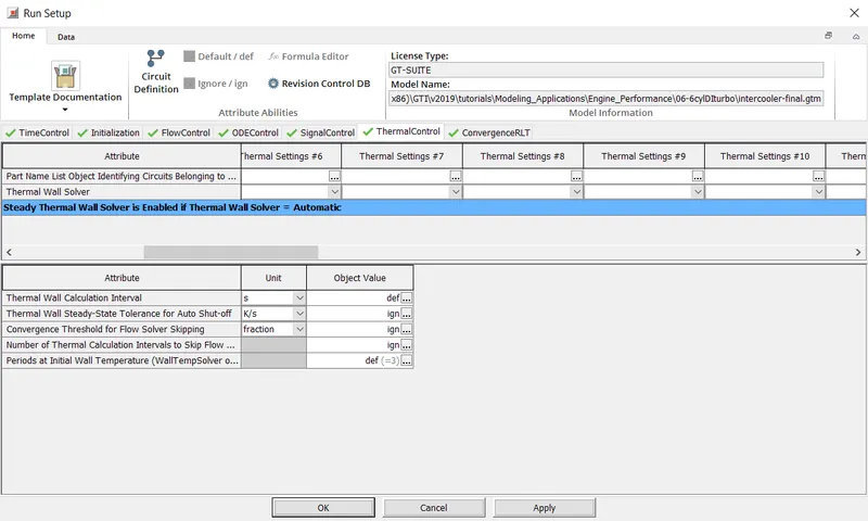
ConvergenceRTL
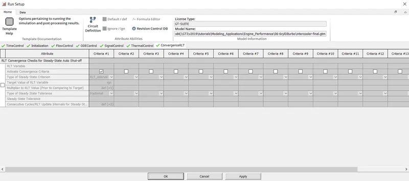
- Advanced Setup
General
Flow
Mechanics
Restart
Version Change
Paths
MiscFiles
- Plot Setup
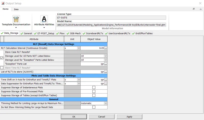
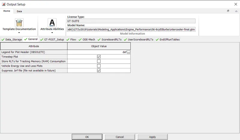
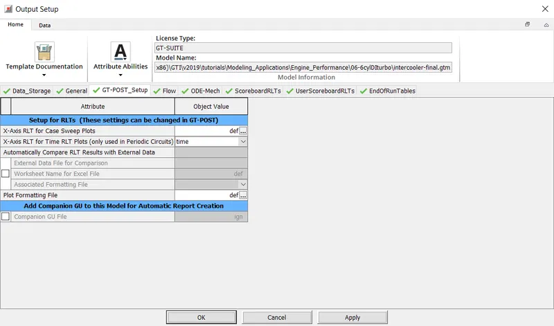
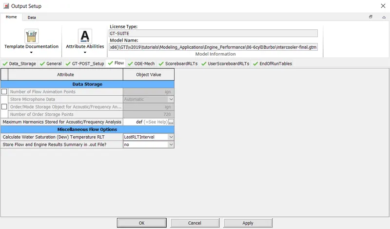
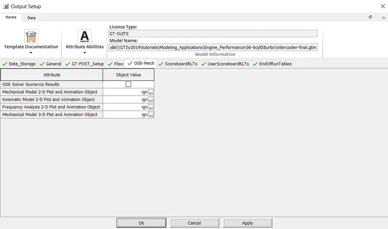
- Output Setup
Data Storage
General
GT-Post Setup
Flow
ODE Mech
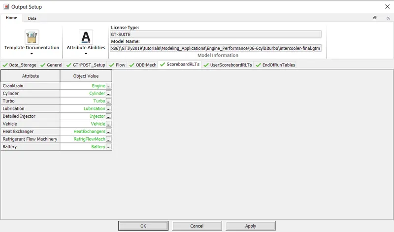
Scoreboard RLTs
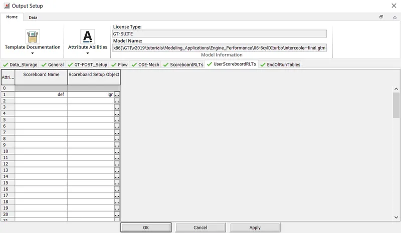
User Scoreboard RLTs
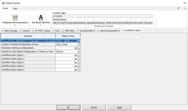
End Of Run Tables
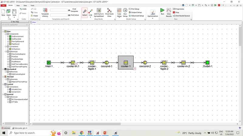
4.To simulate an Intercooler and to calculate the average heat transfer rate and pressure drop across the system.
Given
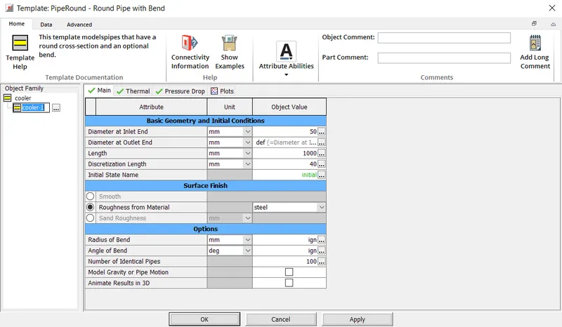
- Diameter of cooler inlet and outlet pipe= 50 mm
- Length of the CAC= 1000 mm
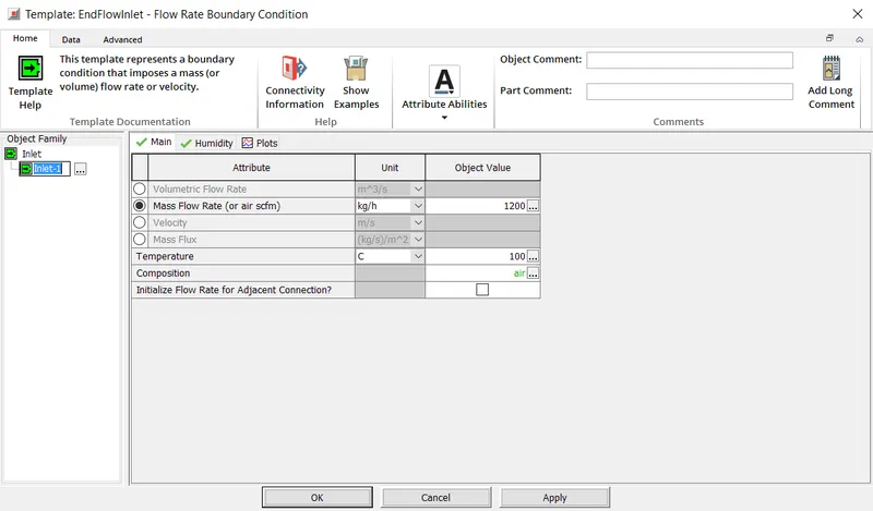
- Inlet mass flow rate = 1200 kg/ h at 100 degC
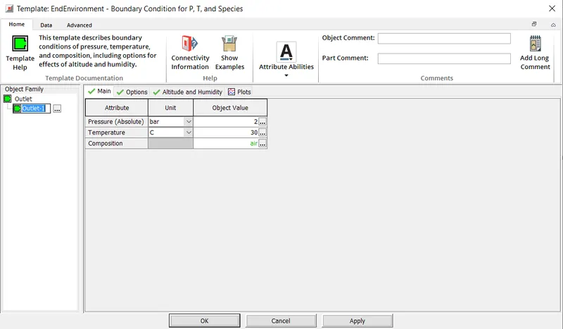
- Outlet pressure 2 bar at 30 deg C
To Find:
- Calculate the Average heat transfer at Charge air cooler (CAC)
- Calculate pressure drop across CAC
An intercooler is a heat exchanger used to cool a gas.Often found in turbocharged engines, intercoolers are also used in air compressors, air conditioners, refrigeration and gas turbines.
Pre Processing
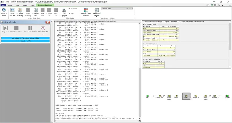
Solver
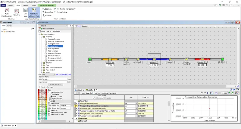
Post Processing
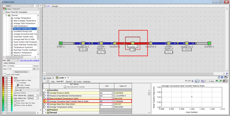
Results
Pressure Drop across Charge Air Cooler : 0.0000112 Bar
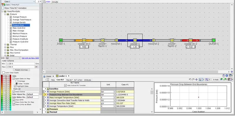
Average Heat Transfer Rate of Charge Air Cooler: 7.55kW
Conclusion:
Through this Challenge, the GUI of the GT-Suite was explored and the different settings were studied. Also the Intercooler System was simulated and the results were extracted.