Week 1: Channel flow simulation using CONVERGE CFD

1. Title – Channel Flow Simulation

2. Objective –

• To create the model of channel in converge Software.
• To set up the case with proper grid size, material and boundary conditions.
• To solver the case using Cygwin terminal and convert the result for Paraview software.
• To import output files in Paraview and generate required contours and plots.

3. Introduction –

Computational Fluid Dynamics (CFD) is the analysis of fluid flows using numerical solution methods. Using CFD, you are able to analyse complex problems involving fluid-fluid, fluid-solid or fluid-gas interaction. Engineering fields where CFD analyses are frequently used are for example aerodynamics and hydrodynamics, where quantities such as lift and drag or field properties as pressures and velocities are obtained. Fluid dynamics is involved with physical laws in the form of partial differential equations. Sophisticated CFD solvers transform these laws into algebraical equations and are able to efficiently solve these equations numerically.

CONVERGE CFD software has a plethora of powerful and flexible features to help us obtain accurate and efficient results for a vast array of general flow problems. From refining dirty CAD geometries to post-processing simulation data, CONVERGE offers a range of features to make our engineering design and analysis life easy. With its powerful tools, CONVERGE can easily handle complex geometries and simulate moving boundaries.

4. Theory –

Flows in conduits or channels are of interest in science, engineering, and everyday life. Flows in closed conduits or channels, like pipes or air ducts, are entirely in contact with rigid boundaries. Most closed conduits in engineering applications are either circular or rectangular in cross section. Open-channel flows, on the other hand, are those whose boundaries are not entirely a solid and rigid material; the other part of the boundary of such flows may be another fluid, or nothing at all. Important open-channel flows are rivers, tidal currents, irrigation canals, or sheets of water running across the ground surface after a rain.

In this simulation we will study flow in close channel and analyse the flow profile, velocity and pressure value at three different mesh size. Flow will be assumed as laminar with steady state. Navier- stokes equation will be used to find the fluid parameter by the solver.

5. Procedure –

There are three major steps in any CFD simulation 1. Pre-processing 2. Solving 3. Post-processing. Pre-processor deals with geometry creation and its cleaning, solver contains material definition, solver model type and boundary conditions, it solves the equations. In Post processor data is collected, which is generated by solver and from them, various charts, contours and animations are created. For this simulation the following procedure was followed –

Geometry creation –

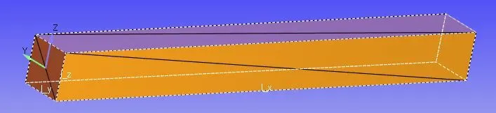
To represent close channel a box was created using option box option in geometry’s create section. The dimensions were given as the following image is showing.

Case setup –

On selecting the option begin case setup, we got the set of the step which needed to follow for the setup. This is a nice feature of converge software with this one can stick to the procedure rigidly. There is a window below geometry which shows the issues, if any, in the geometry and setup. Name boundaries were also given line inlet, outlet etc. Front and back face are kept 2D because, we want to run 2D simulation.

Geometry menu -

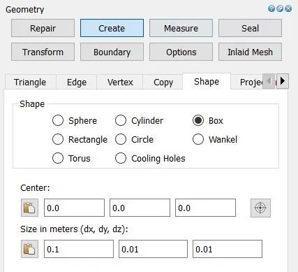
Geometry -

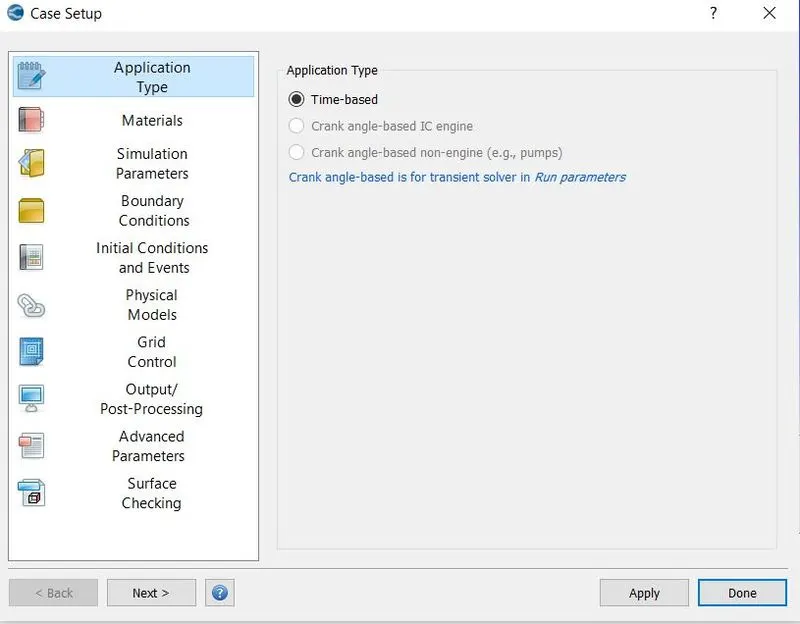
We chose time-based as application type, since it was a simple case and there was no involvement of crank angles.

Case setup menu -

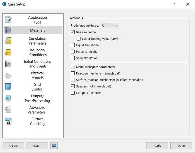
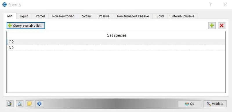
Flowing fluid was assumed air and it is flowing there is no rection or phase change is taking place, that’s why we selected gas simulation with no reaction mechanism. Species O2, N2 was selected.

Material selection -

Species selection -

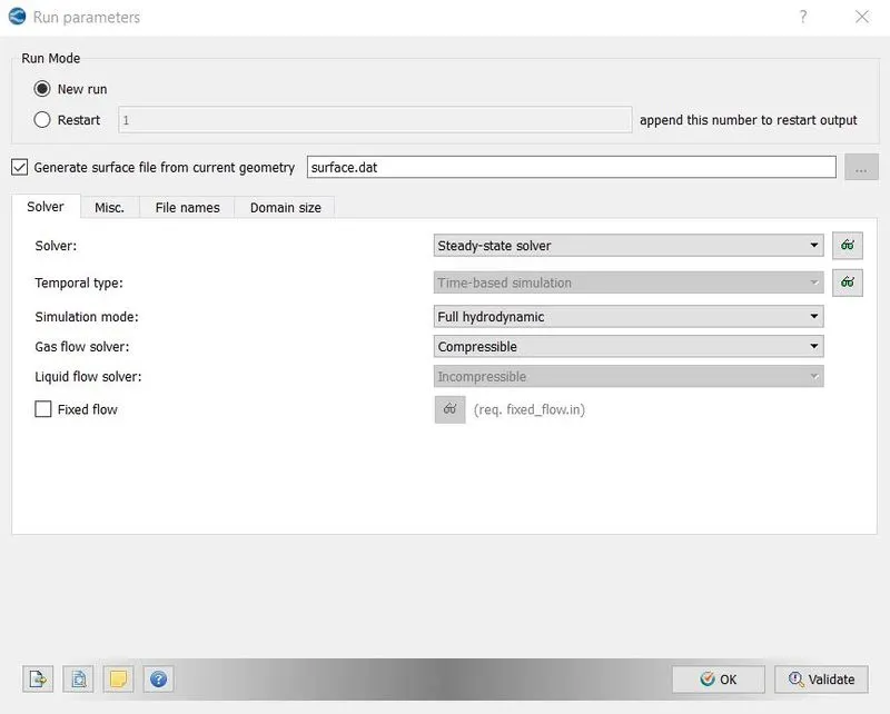
In simulation parameters pressure base steady state with compressible gas flow solver was chosen. Other parameters were kept same.

Run parameters -

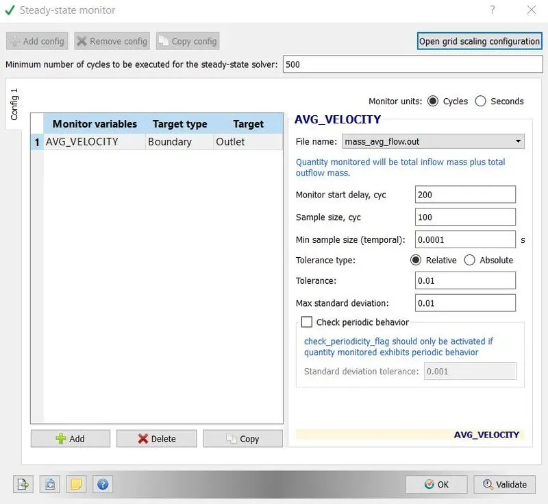
Using steady state monitor we can have eye on the parameters like following image is showing parameter - average velocity at outlet. Pressure, density, temperature can be viewed.

Steady state monitor window -

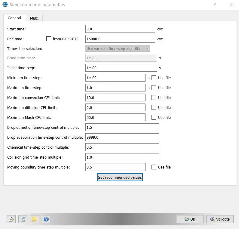
In simulation time parameter starting and end time of simulation, initial, maximum and minimum time step was set. Solver parameters were kept unchanged.

Time parameters -

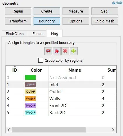
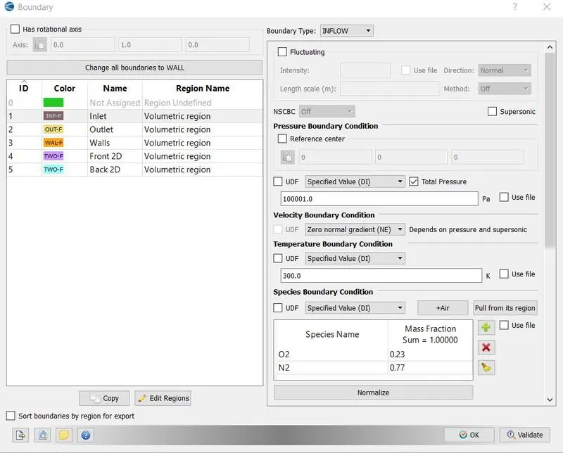
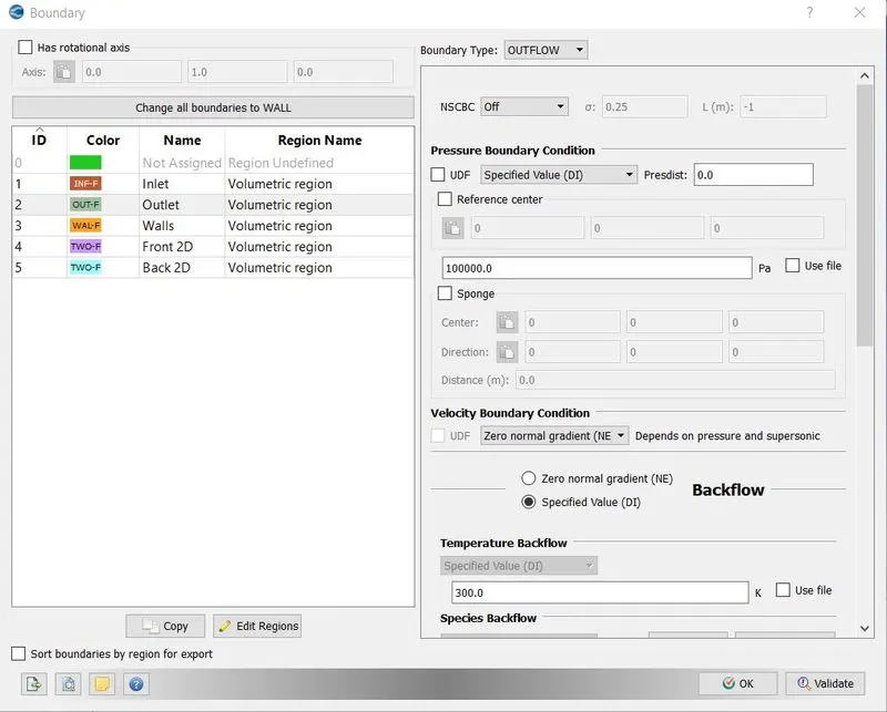
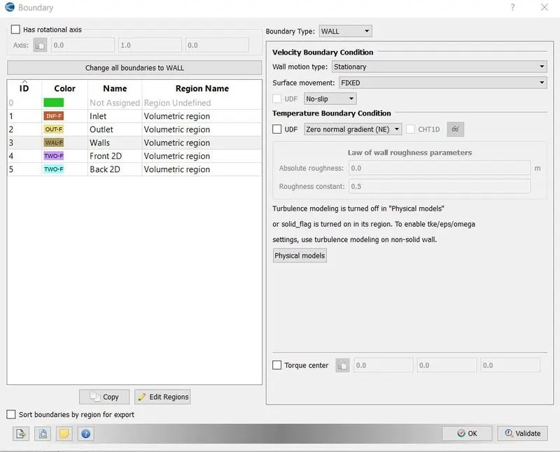
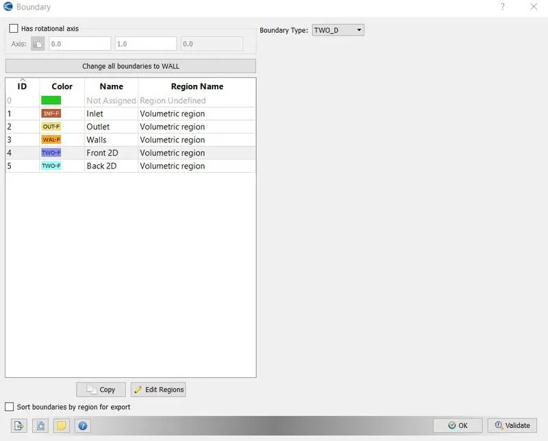
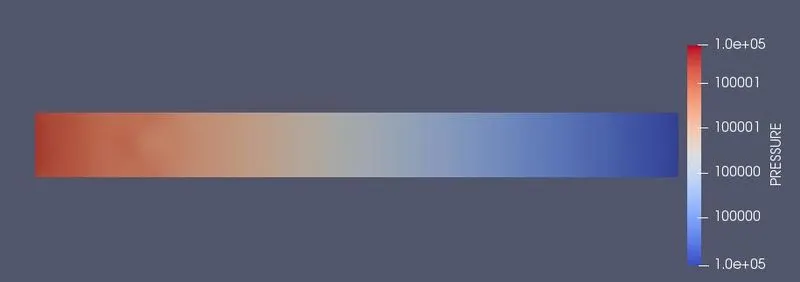
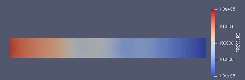
Boundary condition was applied in order to solver Navier-stokes equation. Pressure Difference between in flow and outflow was kept 1 Pascal and this was the reason of flow.

Bonudary selection -

Boundary conditions -

Inlet -

Outlet -

Walls -

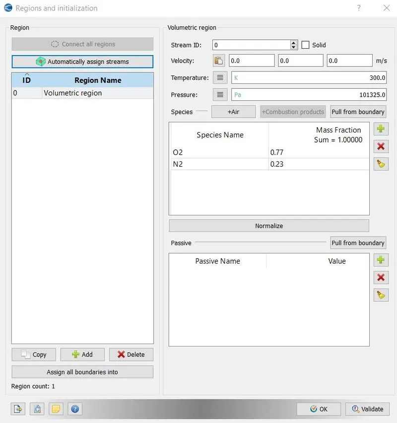
In regions and initialization concentration of O2 and N2 was defined.

Region selection-

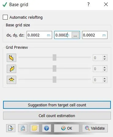
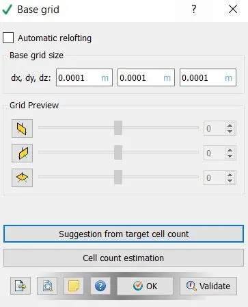
Unchecked the turbulence model parameter because we assumed it as laminar flow. In option base grid meshing size was defined. There were three cases of three different base grids.

Grids setting -

Case1-

Case2-

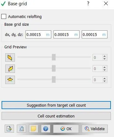
Case3-

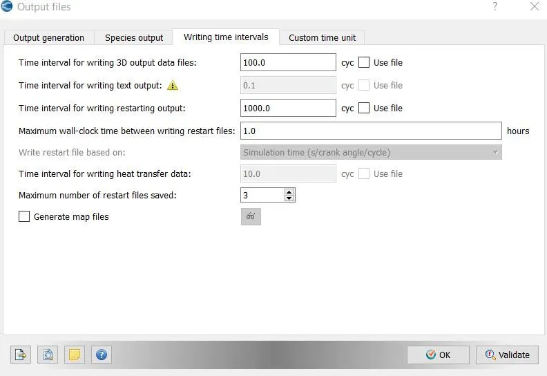
Using post variable selection parameters was selected for which we want data. Using output files option time interval for writing data file and time for restarting was defined. After completing the case setup all files were exported to a folder, from where these can be solved later using Cygwin.

Output setting -

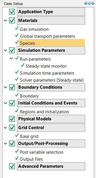
Case Setup (After completing)

Commands used in cygwin -

To Change directory -

cd (path)

To run the simlation -

mpiexec.exe -n 4 converge.exe restricted

To save log files -

mpiexec.exe -n 4 converge.exe </dev/null>(filename).txt &

Solving –

To run simulation Cygwin was opened as administrator and we copied mpiexec and converge executable files the folder, where files were exported after case setup. One can make environment variable for the both executable files, otherwise we have to copy these files in every case. After opening Cygwin directory was changed using cd command and ran mpiexec file and after it converge executable file was run.

Results –

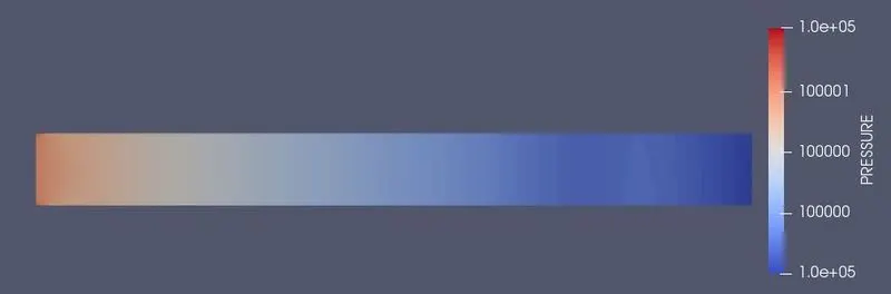
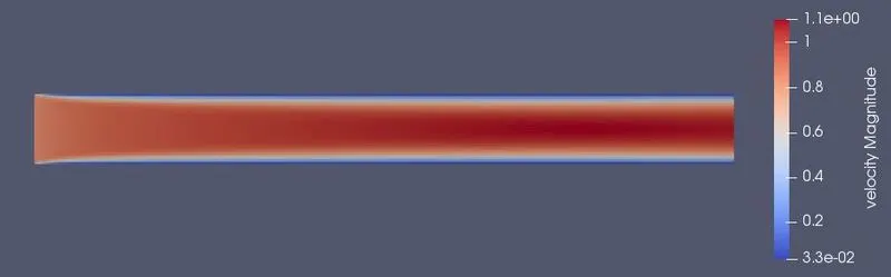
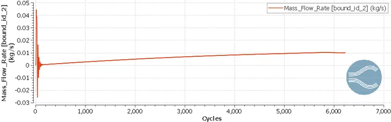
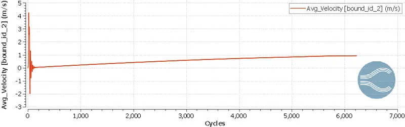
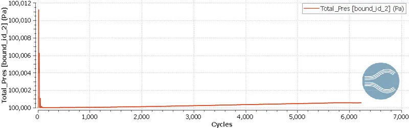
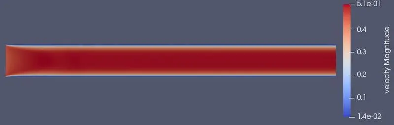
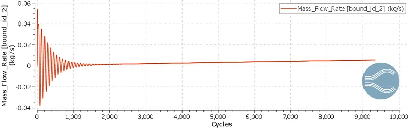
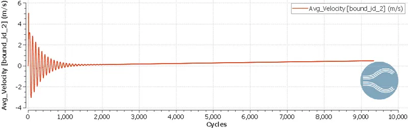
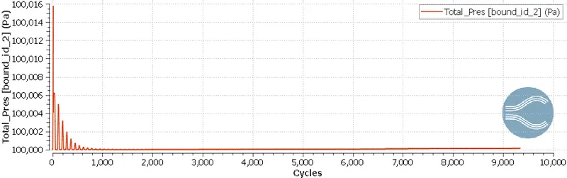
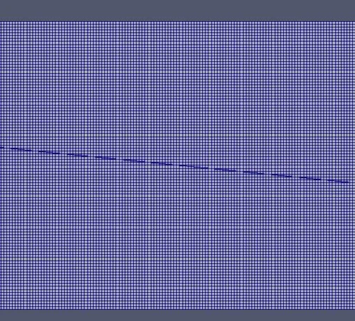
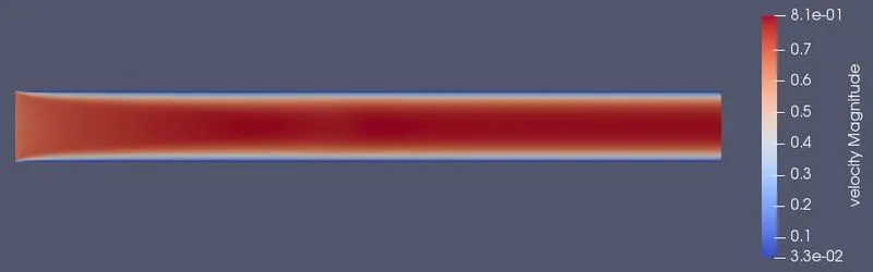
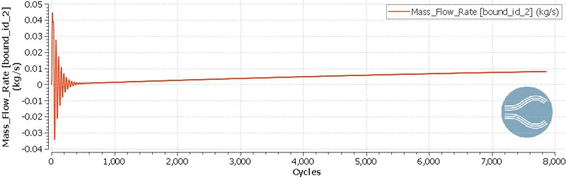
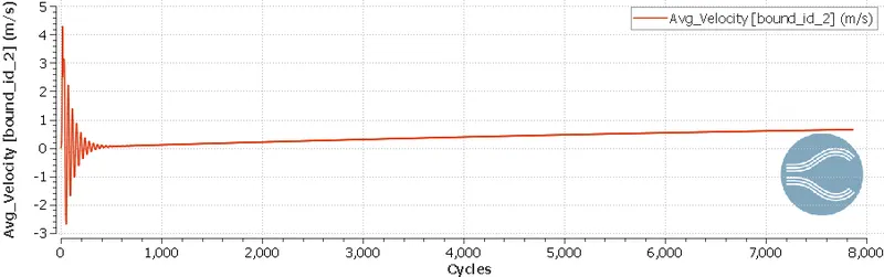
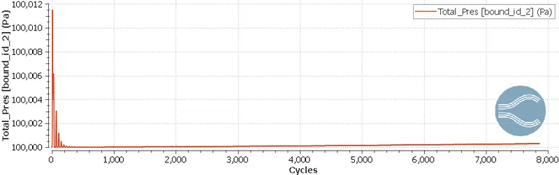
Velocity and pressure contour was created and velocity animation was also created to get good insights of flow and its profile. The pressure difference between inlet and outlet is almost one pascal for all three cases. The value of velocity is varying according grid size, as mesh is getting finer velocity is decreasing. Values of mass flow rate, pressure and velocity are fluctuating at the beginning of simulation and they are converging as the simulation proceeds. By seeing at velocity contour, we can say fluid velocity is following parabolic profile, which is validating theory.

Case1

Mesh -

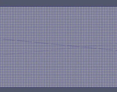
Amination –

https://drive.google.com/file/d/1R21Ty35Ajc8aN9BwR2su3rwTKwHrCUHu/view?usp=sharing

Pressure contour –

Velocity contour –

Mass flow rate plot –

Velocity plot –

Pressure plot –

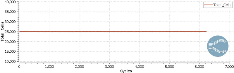
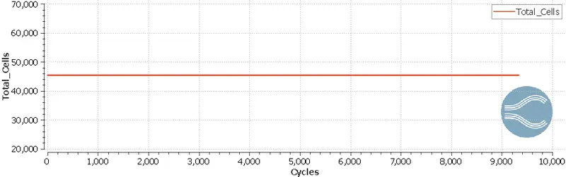
Cell count plot –

Case2

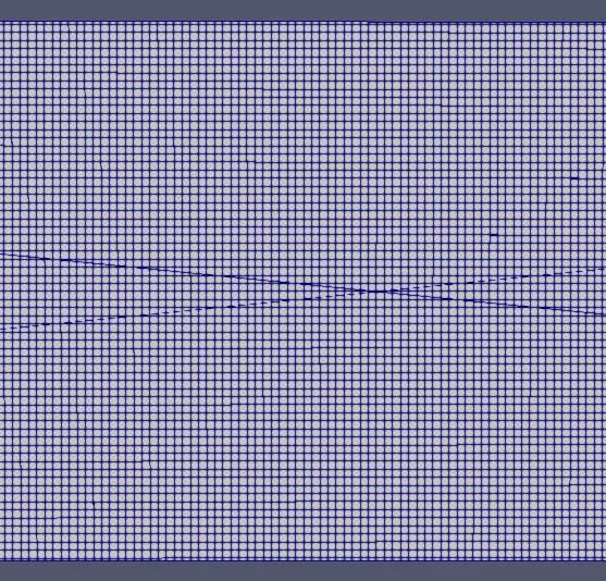
Mesh -

Amination – https://drive.google.com/file/d/1oUun56EEoKZHESdPP3bLENw49f4LEI7w/view?usp=sharing

Pressure contour –

Velocity contour –

Mass flow rate plot –

Velocity plot –

Pressure plot –

Cell count plot –

Case3

Mesh -

Amination –

https://drive.google.com/file/d/1VulZJbsSvz8RlRqPcWnbvZCoBoqKvAON/view?usp=sharing

Pressure contour –

Velocity contour –

Mass flow rate plot –

Velocity plot –

Pressure plot –

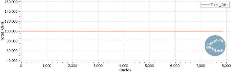
Cell count plot –

Results at a glance –

Case no./Parameters	Number of Cells	Maximum Velocity (m/s)	Mass flow rate (Kg/s)
Case1	25000	1	0.01
Case2	46000	0.51	0.0095
Case3	100,000	0.8	0.0080

6. Conclusion –

Converge software has an important role in CFD simulation specifically in IC engine simulation. It is very fast and very to update. In this study we simulated flow in close channel and generated some result, on the bases of those we conclude that as mesh becomes finer parabolic profile of velocity is getting visibility, if we talk about velocity profile of some other contours, finer mesh always helps in terms of visibly, it does not mean that finer mesh produces better results than coarser one, always. Pressure is difference is the only cause of fluid flow here and it can be seen on pressure contour.