Week 1: Channel flow simulation using CONVERGE CFD
Aim:- To simulate the flow of air through a channel using converge CFD.
Theory:-
The flow-through channels are basically of 2 types:
1. Open channel flow: In this type, the flow is only for liquids. Here the flow with a free surface opens to the atmosphere.
2. Closed channel flow: Example pipe flow, Flow of air through the duct, closed rectangular channel.
The CFD simulation is obtained by solving the Navier-Stokes equations. These are 5 equations continuity, momentum(3 equations), and energy equation. The continuity, momentum equations are solved for all types of flow problems, and the energy equation is used only when heat transfer is taking place to speed up the simulation. These equations are numerically solved in computers by using algorithms like SIMPLE and PISO.
SIMPLE:
SIMPLE stands for Semi Implicit Method for Pressure Linked Equation. This algorithm is only used for steady-state problems. This method works on the pressure correction method. In the first step where the pressure is guessed and termed as the predictor step and the next step where the corrections are applied is termed as the corrector step. In the SIMPLE algorithm, there is 1 predictor and corrector step in each iteration. This iteration run carries until the average change over multiple iterations is less than a tolerance value.
The pressure at step n+1 is given by `p^(n+1) = p^(*****)+ ap^n`
where a is an under relaxation factor whose value is 0 to 1.
PISO:
PISO stands for Pressure Implicit with Splitting of Operator. This is used for both steady and transient state problems. PISO is similar to the SIMPLE whereas SIMPLE uses 1 corrector step and PISO uses 2 or more corrector steps. This algorithm allows larger time steps without affecting the stability of the solution.
Case Setup:
1. Creating the Geometry and boundaries:
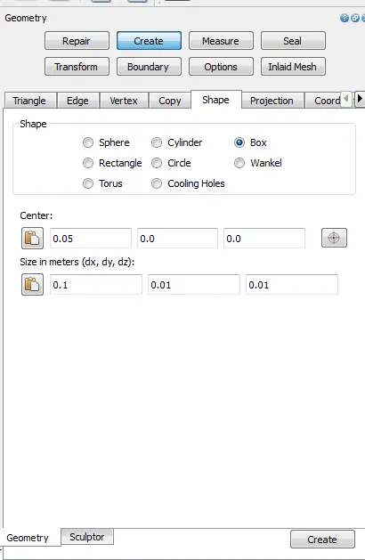
Go to geometry editing toolbox > create > shape > box and enter the values of center and dimensions of dx, dy, and dz to create the geometry. After that in the geometry toolbox select boundary > flag > select +ion.
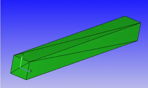
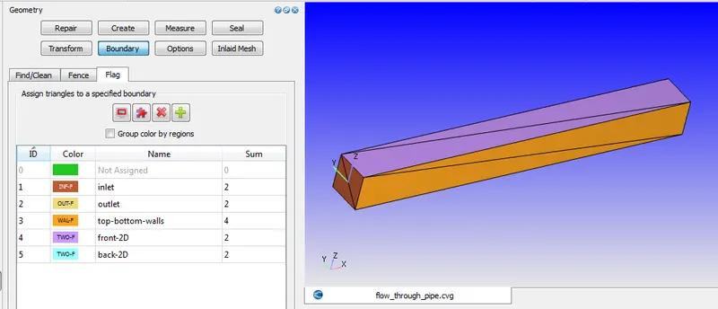
A new window named boundary definition will appear and create the number of boundaries we require and click apply. Assign the boundaries to the 6 faces of the channel(each face contains 2 triangles) and rename the boundaries as inlet, outlet, top-bottom walls, front 2D, and back 2D.
2. Check the orientation of normals:
Enable the normals by clicking the normal toggle icon which is located on the bottom side in the left panel. Actually, the normals should be pointed towards the flow of fluid or air in the channel but here the normals are pointed reversed as shown in the below figure.
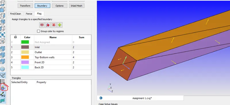
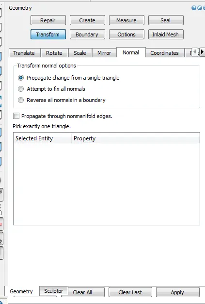
To avoid this select any triangle on the face whose normal is pointed away from the flow and select transform in the geometry toolbox > normal > click on propagate change from single triangle and press apply.
3. Run the diagnosis, for geometry errors
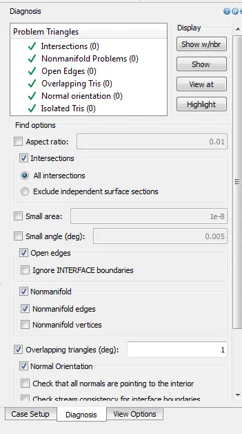
Click on diagnosis which is located on the right side of the panel. If all the parameters are having a green tick mark then there are no errors in the geometry.
4. Go to case setup:
The case setup tab is located beside the diagnosis tab on the right side of the panel.
4.1 Application type:
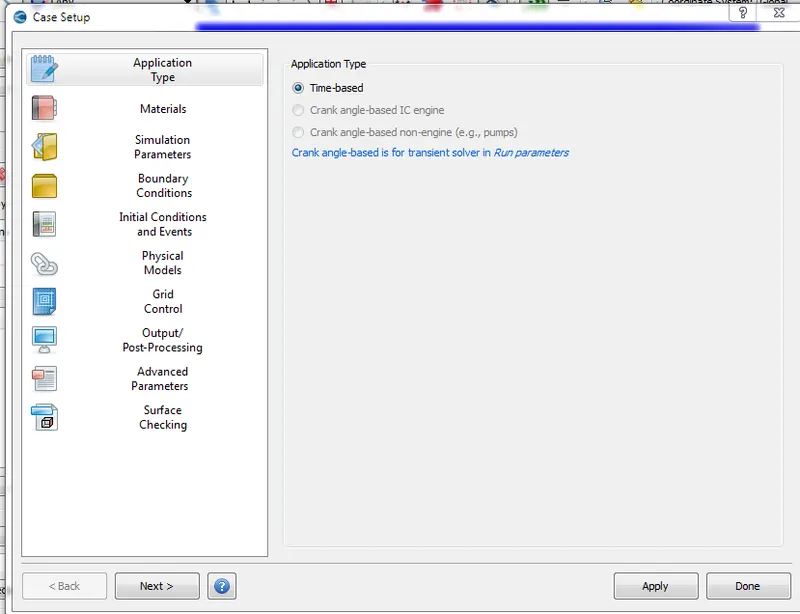
Select application type > Time-based > apply.
4.2 Materials:
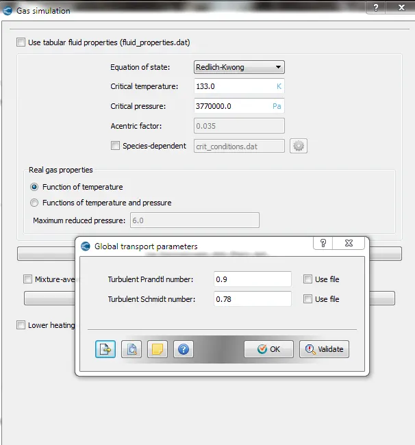
i. Gas simulation:
ii. Global Transport properties:
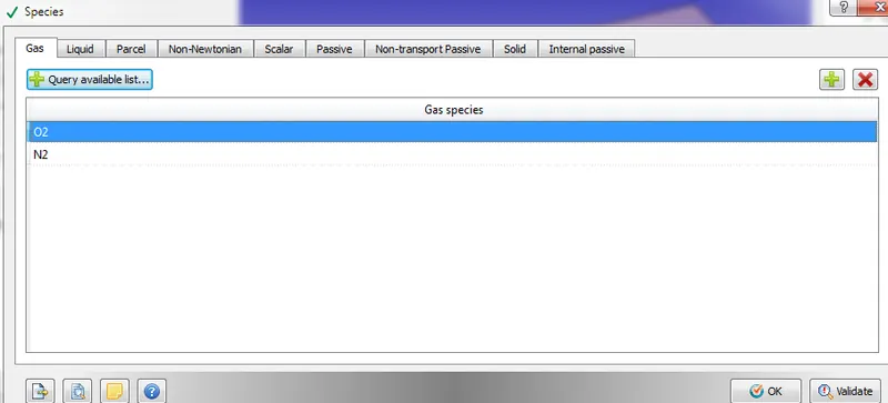
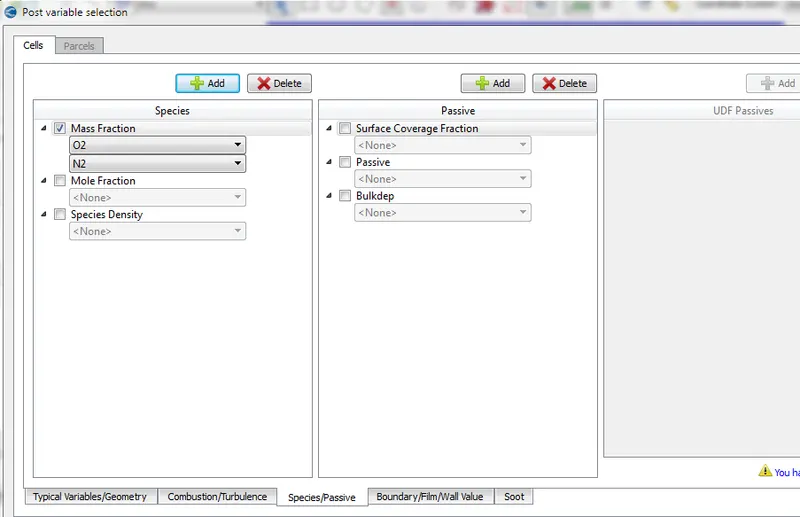
iii. Species: Click on gas > query available list and select oxygen and nitrogen.
4.3 Simulation Parameters:
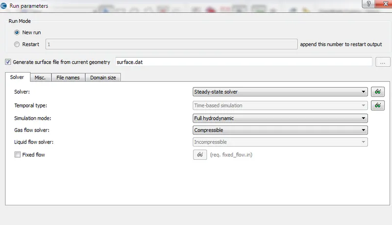
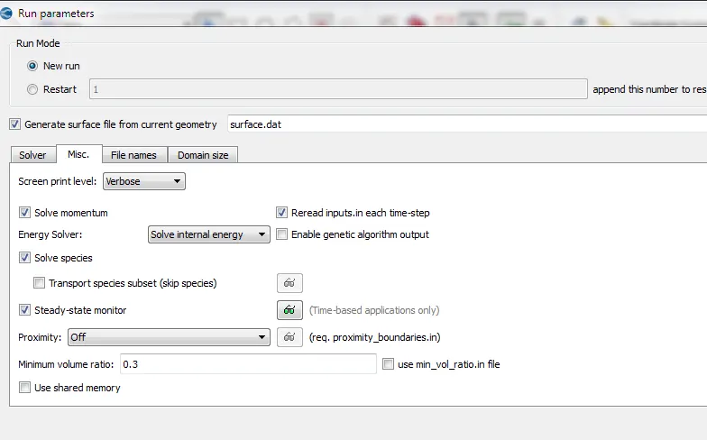
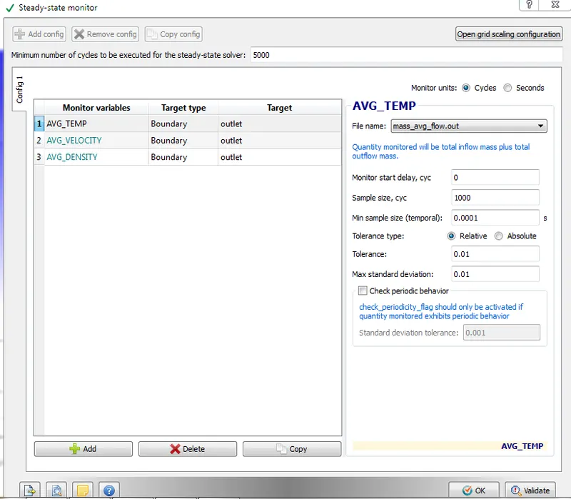
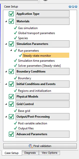
i. Run parameters: Here we are using a steady state solver. And full hydrodynamic because it generates mesh. Coming to misc. untick the shared memory and when we use steady-state solver tick the steady-state monitor.
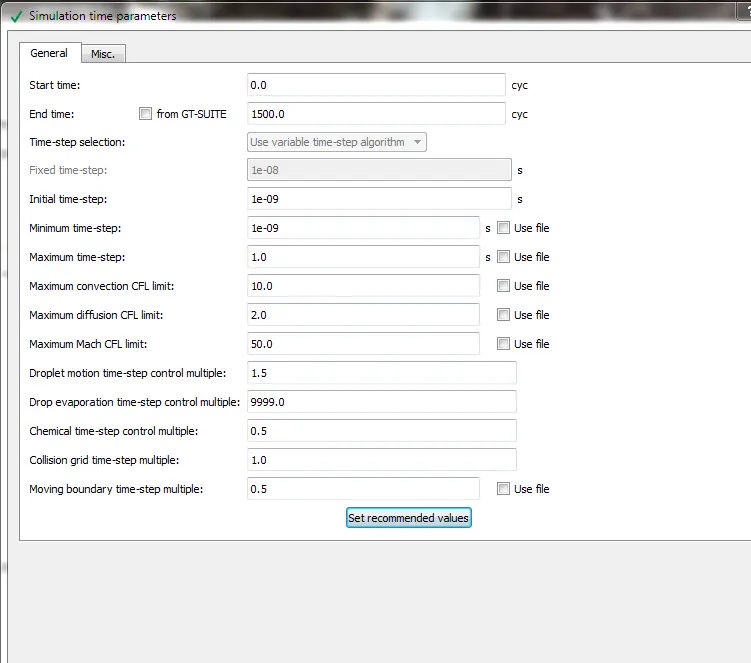
ii. Simulation time parameters:
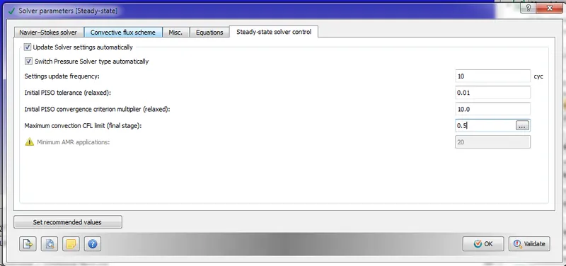
iii. Solver parameters: The value for the maximum convection CFL limit should be less than one.
4.4 Boundary Conditions:
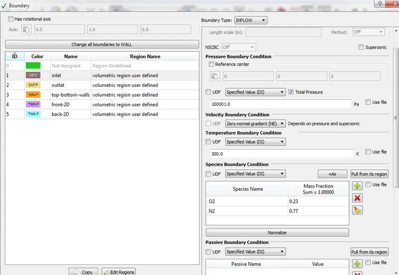
Select the volumetric region user-defined in the region name which was created in the initial conditions and events. Select boundary type Inflow for inlet, Outflow for an outlet, walls for top-bottom walls, and TWO_D for front-2d and back-2d. The remaining pressure, velocity, and species boundary conditions are the same for all boundaries. Add species in the species boundary conditions, where the sum of the total mass fraction should be equal to 1. Here we are using just 2 species(O2 and N2).
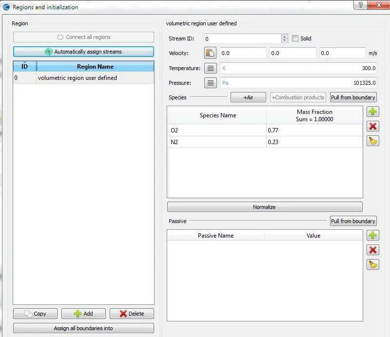
4.5 Initial conditions and events:
4.6 Physical Models:
Disable the turbulence modeling, then select apply.
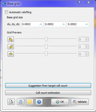
4.7 Grid Control: For meshing, we have to mention the values of dx, dy, and dz in the base grid size > click ok. Here in the challenge, we have 3 different mesh grid sizes as 2e-4, 1.5e-4, and 1.2e-4.
4.8 Output/post-processing:
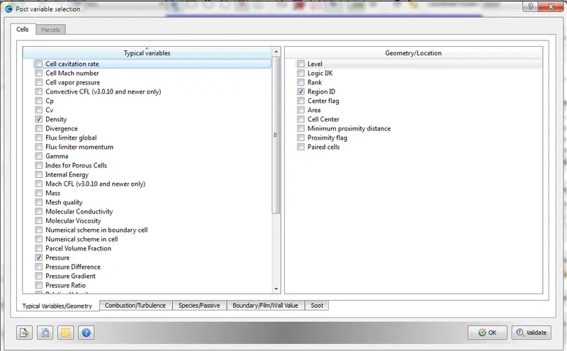
i. Post variable selection: Comming to the combustion/turbulence just untick all turbulence.
ii. Output files:
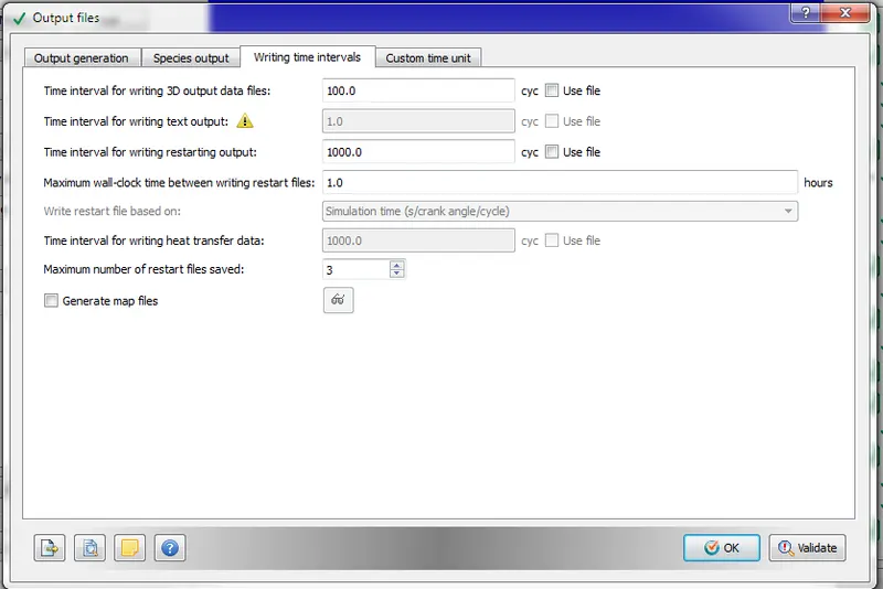
By the end, the case setup should look like this which is shown below:
5. Export all input files into a folder:
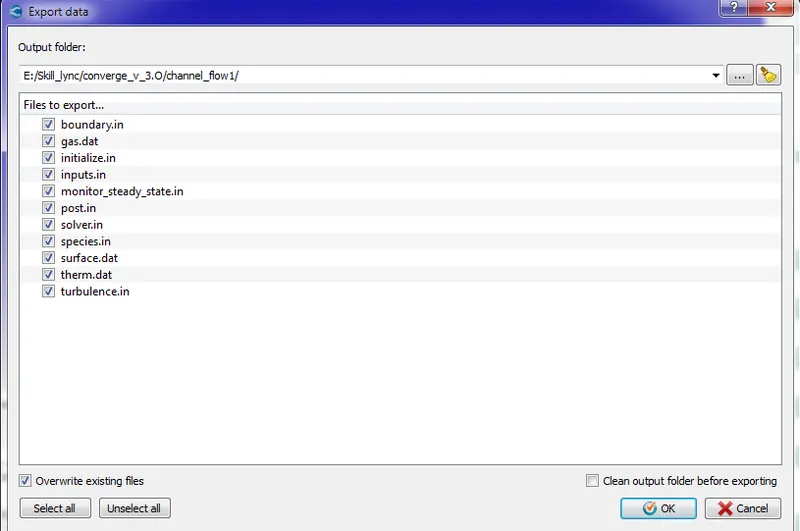
Click on files > Export > Export input files > choose the path and select all files and press ok.
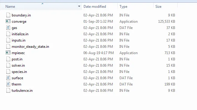
6. Copy and paste the mpiexec.exe file, converge file to the folder in which the input files are exported: The mpiexec.exe file is located at drive c > program files > Convergent_Science > CONVERGE > 3.0.16 > bin > mpi > intel64 > bin. The converge file is located at drive c > program files > Convergent_Science > CONVERGE > 3.0.16 > bin > intelmpi.
7. To run the simulation, open Cygwin:
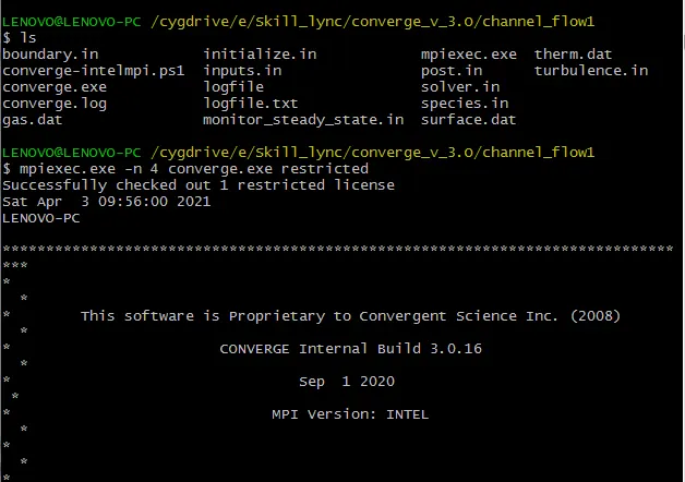
Open Cygwin and navigate to the folder in which the input files are exported and run the command as mpiexec.exe -n 4 converge.exe restricted then press enter the simulation will run automatically.
8. Post-convert all the output files:
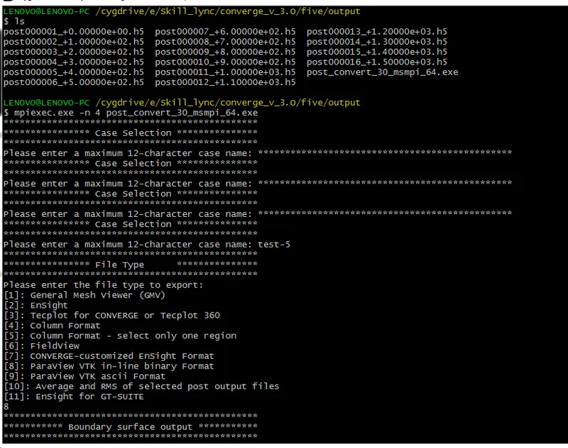
Copy the post_convert_30_msmpi_64.exe file and paste it into the output folder. Now open Cygwin and go to the output folder and type mpiexec.exe -n 4 post_convert_30_msmpi_64.exe > enter the case name > select file type as Paraview VTK in-line binary format > type all for files and cell variables and click enter.
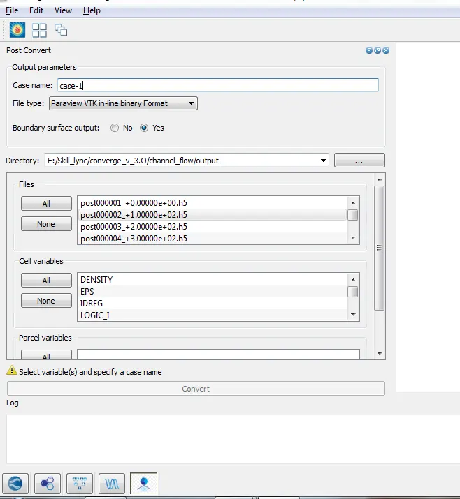
Or we can convert output files in converge-studio, on the bottom left, select the last icon to post-convert the output files. Enter the case name as test and select file type as Paraview VTK in-line binary format. In the directory, select the output folder and copy that location and paste in the directory > select all in files and cell variables > convert.
9. Post-processing the files:
Lanch paraview and open it then open the file location as case1 which is saved in output > case1 .. vtm (this is a group file which is formed during post-converting the files) > click on apply > create a slice along the z-axis.
Results:
For dx=dy=dz=2e-4:
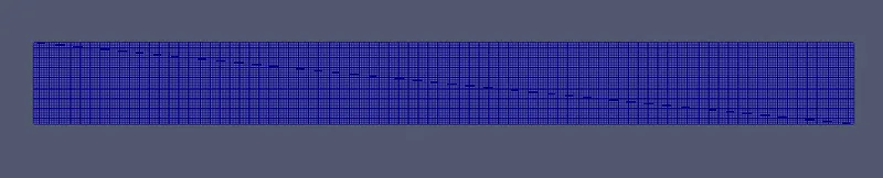
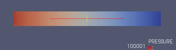
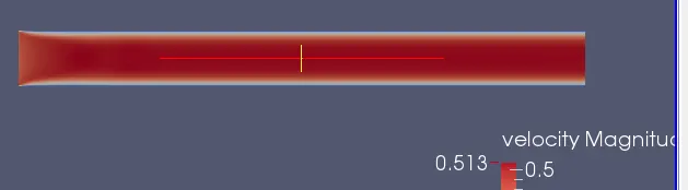
Pressure and Velocity countors:
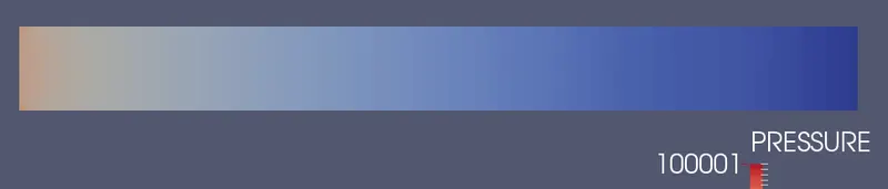
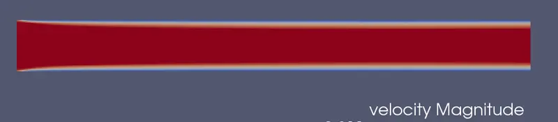
Pressure plot:
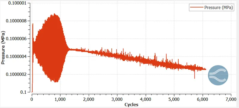
Mass flow rate plot:
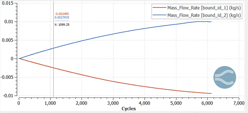
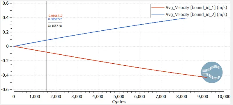
Velocity:
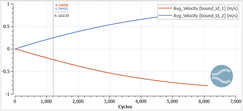
Total cells:
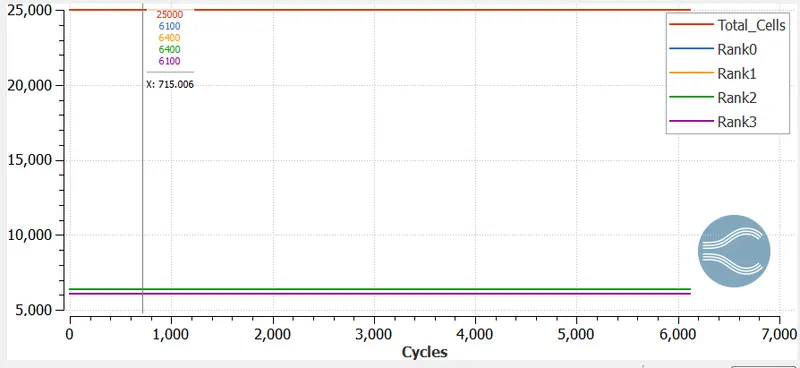
Total cells: 25000
For dx=dy=dz=1.5e-4:
Pressure and Velocity countors:
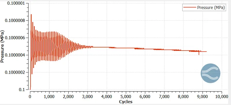
Pressure plot:
Mass flow rate plot:
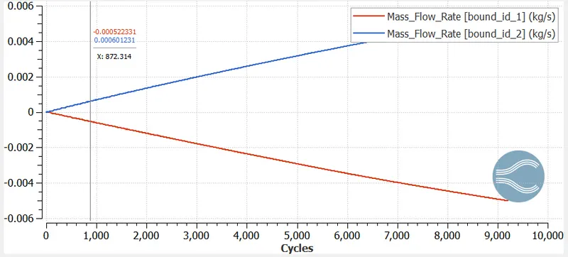
Velocity:
Total cells:
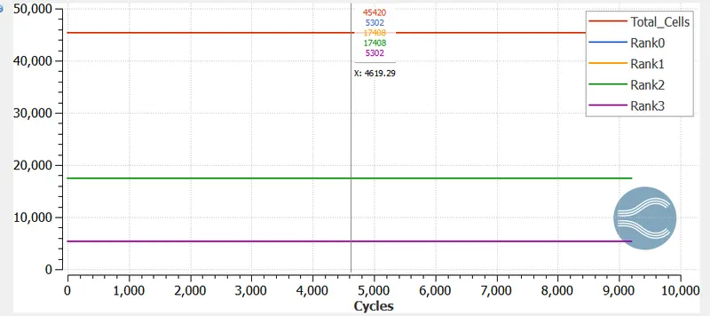
Total cells: 45420
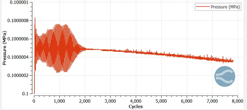
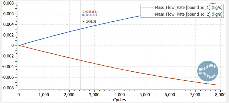
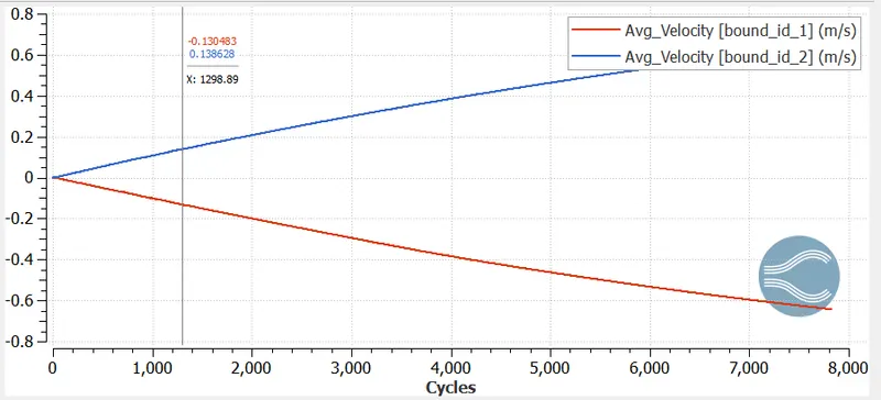
For dx=dy=dz=1.0e-4:
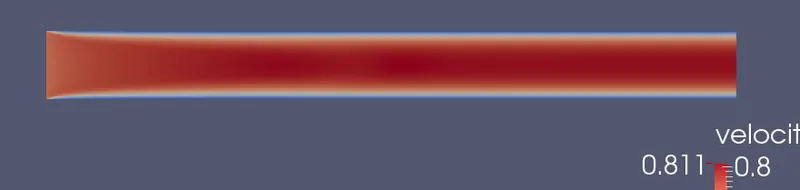
Pressure and Velocity countors:
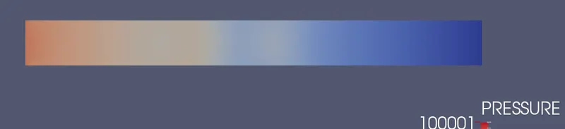
Pressure plot:
Mass flow rate plot:
Velocity:
Total cells:
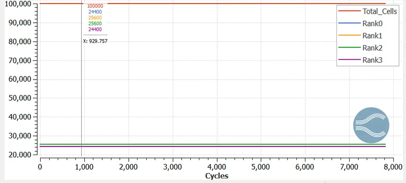
Total cells: 70056
Animation link for 2e-4:
https://www.youtube.com/watch?v=gZLvzLJdMoo&ab_channel=Harsha
Conclusion:
- If the grid size decreases then the total cell count increases and the simulation time also increases. Then we can get accurate results and smooth plots.
- If the mesh size decreases, the converge decreases the time step to maintain the CFL number.