Understanding the stability analysis in linear systems

Consider the following system of matrices.

Coefficient Matrix, A=[5 1 2 ; -3 9 4; 1 2 -7]

Solution Matrix, X=[x1;x2;x3]

Residual Matrix, B=[10 -14 33]

EXPECTED RESULTS :

• Solve the system of matrices using Jacobi, Gauss-seidel and SOR methods.
• Compute the Iteration Matrix for the above mentioned methods by suitable matrix decomposition techniques taught in the lectures.
• Calculate the Eigen values of the Iteration matrix.
• Calculate the Spectral radius of the Iteration matrix.

1) Explain the concept of Eigen value & Spectral radius of the matrix. How does it affect the convergence rate of the solution?

2) What is Diagonal dominance? How do the diagonal terms of an Iteration matrix affect the solution through iterative methods? Is there a relationship between Diagonal dominance and spectral radius ?

[HINT] : Introduce a suitable scaling factor called diagonal magnification factor that scales the given diagonal elements within a range, say [0.1:0.1:2] for answering question 2)

Note: You cannot use the inbuilt functions that are available in Matlab for the calculation of Eigen values of a matrix. Write a detailed explanation for your results, plots or codes without explanation will awarded zero marks.

System of matrices

Coefficient Matrix, A=[5 1 2 ; -3 9 4; 1 2 -7]

Solution Matrix, X=[x1;x2;x3]

Residual Matrix, B=[10; -14; 33]

Aim

• To solve the system of matrices using Jacobi, Gauss-seidel and SOR methods.
• To compute the Iteration Matrix for the above mentioned methods by suitable matrix decomposition techniques.
• To calculate the Eigen values of the Iteration matrix.
• To calculate the Spectral radius of the Iteration matrix.
• To explain the concept of Eigen value & Spectral radius of the matrix and its effect on the convergence rate of the solution.
• To derive a relationship between Diagonal dominance and spectral radius.

Solution

Diagonal matrix=D

Diagonal magnification=dm=0.1:0.1:2

`Dm=D*dm`

Only a single value of dm is passed in each loop.

Lower triangular matrix=L

Upper triangular martrix=U

Identity matrix = I

Jacobi method

`X^(NEW)=Dm^(-1)*(B-((L+U)*X^(OLD)))`

Iteration matrix,

`T=-Dm^(-1)*(L+U)*X^(OLD)`

Gauss seidel method

`X^(NEW)=(L+Dm)^(-1)*(B-(U*X^(OLD)))`

Iteration matrix,

`T=-(L+Dm)^(-1)*U`

SOR method

`X^(NEW)=omega*(L+Dm)^(-1)*B-(I-omega*((L+Dm)^(-1)*U+I))*X^(OLD)`

Iteration matrix,

`T=I-omega*((L+Dm)^(-1)*U+I))`

Matlab code

Main program

clear all
close all
clc

%Understanding stability analysis of linear system

A=[5 1 2 ; -3 9 4; 1 2 -7];
B=[10; -14; 33];

%Traingular matrix separaton (matrix decomposition)

D=diag(diag(A));
L=[0 0 0 ; -3 0 0 ; 1 2 0];
U=[0 1 2 ; 0 0 4 ; 0 0 0];

dm=0.1:0.1:2; %Diaginal magnification

for i=1:length(dm)
    Dm=D*dm(i);

[jacobi_iter(i),x_jac(i,:),jac_error,jacobi_spectral_radius(i)]=jacobi(Dm,L,U,B);

[gs_iter(i),x_gs(i,:),gs_error,gs_spectral_radius(i)]=gs(Dm,L,U,B);

[sor_iter(i),x_sor(i,:),sor_error,sor_spectral_radius(i)]=sor(Dm,L,U,B);
end

%Error calculation
fprintf('Error calculated using Jacobi method=%d',jac_error)
fprintf('n Error calculated using Gauss seidel method=%d',gs_error)
fprintf('n Error calculated using SOR method=%d',sor_error)

%Plots
figure(1)
title('Jacobi method')
subplot(2,1,1)
plot(dm,jacobi_spectral_radius)
xlabel('Diagonal magnification')
ylabel('Spectral radius')
axis([0 2 0 2])
grid on
subplot(2,1,2)
plot(jacobi_spectral_radius,jacobi_iter,'color','r')
xlabel('Spectral radius')
ylabel('No of iterations')
axis([0 1.5 0 100])
grid on

figure(2)
title('Gauss seidel method')
subplot(2,1,1)
plot(dm,gs_spectral_radius)
xlabel('Diagonal magnification')
ylabel('Spectral radius')
axis([0 2 0 2])
grid on
subplot(2,1,2)
plot(gs_spectral_radius,gs_iter,'color','r')
xlabel('Spectral radius')
ylabel('No of iterations')
axis([0 1.5 0 100])
grid on

figure(3)
title('SOR method')
subplot(2,1,1)
plot(dm,sor_spectral_radius)
xlabel('Diagonal magnification')
ylabel('Spectral radius')
axis([0 2 0 2])
grid on
subplot(2,1,2)
plot(sor_spectral_radius,sor_iter,'color','r')
xlabel('Spectral radius')
ylabel('No of iterations')
axis([0 1.5 0 100])
grid on

Function codes

Jacobi method

function [jacobi_iter,x_jac,jac_error,jacobi_spectral_radius]=jacobi(Dm,L,U,B)

%Initialization
x=zeros(3,1);
xold=x;
jac_error=9e9;
tolerance=1e-3;
jacobi_iter=1;

%Iterative matrix
Tjac=-inv(Dm)*(L+U); 

eigen_value=roots(poly(Tjac)); 

%Spectral radius
jacobi_spectral_radius=max(abs(eigen_value)); 

 while (jac_error>tolerance)
    x=inv(Dm)*(B-((L+U)*xold));
    jac_error=max(abs(x-xold));
    xold=x;
    jacobi_iter=jacobi_iter+1;
  end
x_jac=x;

end

Gauss seidel method

function [gs_iter,x_gs,gs_error,gs_spectral_radius]=gs(Dm,L,U,B)

%Initialization
x=zeros(3,1);
xold=x;
gs_error=9e9;
tolerance=1e-4;
gs_iter=1;

%Iterative matrix
Tgs=-inv(L+Dm)*U; 

eigen_value=roots(poly(Tgs));

%Spectral radius
gs_spectral_radius=max(abs(eigen_value));

while (gs_error>tolerance)
    x=inv(L+Dm)*(B-(U*xold));
    gs_error=max(abs(x-xold));
    xold=x;
    gs_iter=gs_iter+1;
end
x_gs=x;
end

SOR method

function [sor_iter,x_sor,sor_error,sor_spectral_radius]=sor(Dm,L,U,B)

%Initialization
x=zeros(3,1);
xold=x;
omega=1.2;
sor_error=9e9;
tolerance=1e-4;
sor_iter=1;

%Identity matrix
I=[1 0 0;0 1 0;0 0 1];

%Iterative matrix
Tsor=I-omega*((inv(L+Dm))*U+I); 

eigen_value=roots(poly(Tsor)); 

%Spectral radius
sor_spectral_radius=max(abs(eigen_value)); 

while (sor_error>tolerance)
    x=omega*inv(L+Dm)*B-(I-omega*(inv(L+Dm)*U+I))*xold;
    sor_error=max(abs(x-xold));
    xold=x;
    sor_iter=sor_iter+1;
end
x_sor=x;
end

Explanation

• Matrix values for A, B, D, L, U and diagonal magnification values (dm) are assigned.
• Using 'for loop' upto the length of dm, the functions jacobi, gauss seidel and SOR methods are evaluated.
• For each loop, diagonal matrix with diagonal magnification (Dm) is calculated. (each value of dm is passed per loop)
• In jacobi function, the initial values of x, xold, error, tolerance and iteration number are assigned.
• Then the iterative matrix, eigen value and spectral radius values are computed.
• Inside while loop, the x value, error are computed. The old x values are updated inside the loop and iteration value is incremented. The while loop is executed again and again till the error value falls below the tolerance value.
• When error value falls below the tolerance value, the loop ends and the the x value is assigned to x_jac. The function ends and passes iteration number, error , x_jac and spectral radius value to the main function.
• The same procedure is repeated for gauss seidel and SOR methods with their respective iterative matrix and x values.
• The error values computed in the three methods are printed in the command window using fprintf command.
• The diagonal magnification- spectral radius subplot and the spectral radius- no. of iterations subplots are derived and their respective lables, grids and axis are given.

Output

Error calculated using Jacobi method=6.615255e-04
Error calculated using Gauss seidel method=5.052601e-05
Error calculated using SOR method=8.155802e-05

Plots

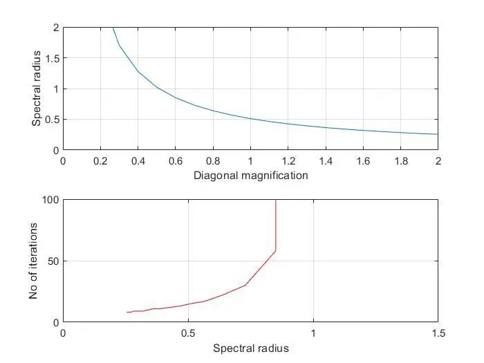
Jacobi method

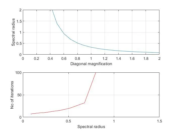
Gauss seidel method

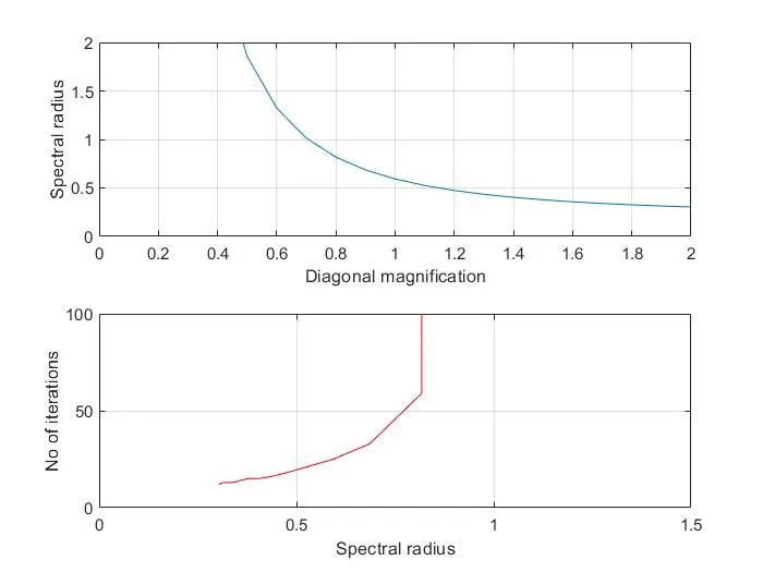
SOR Method

Explanation

In plots each methods, the diagonal magnification(in x-axis)- spectral radius (in y-axis) subplot and the spectral radius (in x-axis) - no. of iterations subplots (in y-axis) are obtained. When diagonal magnification increases, spectral radius value decreases.

When spectral radius value increases, the no. of iterations required to converge also increases. This is true upto the spectral radius value less than 1.

Concept of Eigen value, Spectral radius of the matrix.

Using poly command to the iteration matrix of the each method (Jacobi, gauss seidel, SOR), yields the coefficient values of the charateristic polynomial. Using roots command to the charateristic polynomial, yields the eigen value of the iteration matrix of the each methods.

The maximum of the absolute value of the eigen value of each methods is the spectral radius.

Diagonal dominance, spectral radius and convergence rate of the soultion

• The matrix is said to be strictly diagonally dominant if and only if the magnitude of diagonal element in a row is greater than the sum of magnitudes of other elements in the row.
• The given matrix A is strictly diagonally dominant.
• Boundedness is the condition for convergence. The spectral radius value of less than 1 and diagonally dominant matrix implies that the solution at all the nodes is bounded (converged).
• From the plots we see that when diagonal magnification increases, spectral radius value decreases. So for higher diagonal magnification values, the spectral radius is smaller (less than 1) and therefore the soultion is stable.

Let us choose a diagonal magnification value in such a way that spectral radius value is greater than 1. Let us replot the no. of iterations(to converge) and spectral radius plot for the three methods with some modifications in axis values (for better understanding)

Jacobi method

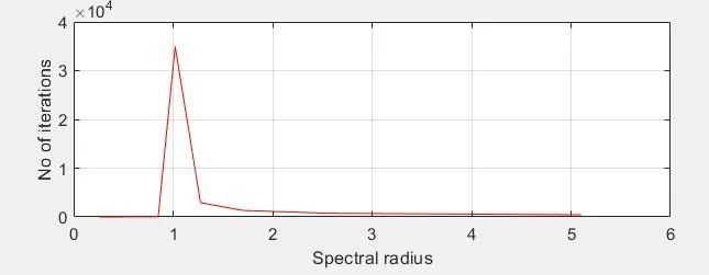
For diagonal magnification value at 0.5, the spectral radius value is 1.02. From the plot, after the spectral radius value of 1.02, the the number of iterations required to converge decreases drastically and the solution becomes unstable.

Gauss seidel method

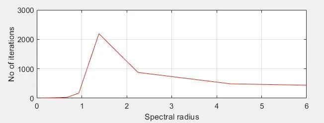
For diagonal magnification value at 0.5, the spectral radius value is 1.381. From the plot, after the spectral radius value of 1.381, the the number of iterations required to converge decreases drastically and the solution becomes unstable.

SOR method

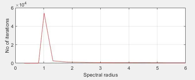
For diagonal magnification value at 0.7, the spectral radius value is 1.013. From the plot, after the spectral radius value of 1.013, the the number of iterations required to converge decreases drastically and the solution becomes unstable.

From the plots we can conclude that when spectral radius is greater than 1, the solution becomes unstable for Jacobi, Gauss seidel and SOR methods.

Conclusion

• Solved the system of matrices using Jacobi, Gauss-seidel and SOR methods.
• Computed the Iteration Matrix for the above mentioned methods by suitable matrix decomposition techniques.
• Calculate the Eigen values of the Iteration matrix for each method.
• Calculate the Spectral radius of the Iteration matrix for each method.
• Explained the concept of Eigen value & Spectral radius of the matrix
• Explained the diagonal dominance, spectral radius and convergence rate of the solution and derived relationship among them.
• The solution is stable when spectral radius is less than 1 and diagonal dominance of matrix (A). It becomes unstable if spectral radius is greater than 1 for all the three methods.