Solving the steady and unsteady 2D heat conduction problem

Aim

To solve the 2D heat conduction equation by using the point iterative techniques using the methods like Jacobi, Gauss-seidel, Successive over-relaxation for both implicit and explicit schemes.

Inputs and boundary conditions

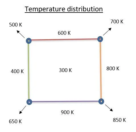
Domain is assumed to be a shape of a square of lenght 1m.

No. of nodes at x and y direction be nx=ny=10.

Temperature at the nodes,

• Top Boundary = 600 K
• Bottom Boundary = 900 K
• Left Boundary = 400 K
• Right Boundary = 800 K
• Initial temperature inside the domain=300 K
• Top left corner = `(600+400)/2=500K`
• Top right corner = `(600+800)/2=700K`
• Bottom left corner = `(900+400)/2=650K`
• Bottom right corner = `(900+800)/2=850K`

Absolute error criteria is 1e-4

Solution

Steady state 2D heat conduction equation

`(del^2T)/(delx^2)+(del^2T)/(dely^2)=0 implies nabla^2T=0`

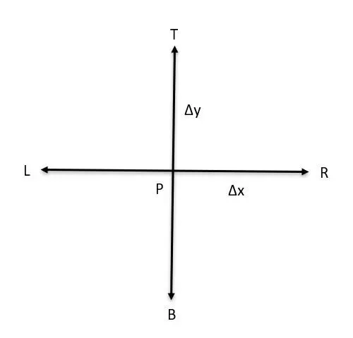
Discretizing the above equation using Central differencing scheme(CDS), we get

`((T underset(L)()-2*Tunderset(p)()+T underset(R)())/(Deltax^2)+(T underset(T)()-2*Tunderset(p)()+T underset(B)())/(Deltay^2))=0`

Futher simplifying the above equation, we get

`T underset(p)()=(1/K)*((T underset(L)()+T underset(R)())/(Deltax^2)+(T underset(T)()+T underset(B)())/(Deltay^2))`

`K=2*((Deltax^2+Deltay^2)/(Deltax^2*Deltay^2))`

Jacobi method

`T underset(p)()^(n+1)=(1/K)*((T underset(L)()+T underset(R)())/(Deltax^2)+(T underset(T)()+T underset(B)())/(Deltay^2))^n`

Gauss seidel method

`T underset(p)()^(n+1)=(1/K)*((T underset(L)()+T underset(R)())/(Deltax^2)+(T underset(T)()+T underset(B)())/(Deltay^2))^(n+1)`

Successive over relaxation method

`T underset(p)()^(n+1)=T underset(p)()^(n)*(1-omega)+omega*((1/K)*((T underset(L)()+T underset(R)())/(Deltax^2)+(T underset(T)()+T underset(B)())/(Deltay^2))^(n+1))`

Transient flow

Explicit approach

`(delT)/(delt)=alpha*((del^2T)/(delx^2)+(del^2T)/(dely^2))`

Discretising the above equations using Forward differencing scheme(FDS) for time derivative and Central differencing scheme(CDS) for space derivative, we get,

`(T underset(p)()^(n+1)-T underset(p)()^(n))/(Deltat)=alpha*((T underset(L)()-2*Tunderset(p)()+T underset(R)())/(Deltax^2)+(T underset(T)()-2*Tunderset(p)()+T underset(B)())/(Deltay^2))^n`

`T underset(p)()^(n+1)=T underset(p)()^(n)+K underset(1)()*(T underset(L)()-2T underset(p)()+T underset(R)())^n +K underset(2)()*(T underset(T)()-2T underset(p)()+T underset(B)())^n`

`T underset(p)()^(n+1)=T underset(p)()^(n)*(1-2*K1-2*K2)+K1*(T underset(L)()+T underset(R)())^n+K2*(T underset(L)()+T underset(R)())^n`

where `K underset(1)()=alpha*(delT)/(delx^2) and K underset(2)()=alpha*(delT)/(dely^2)`

where `CFLunderset(x)()=Kunderset(1)() and CFLunderset(y)()=Kunderset(2)()`

For explicit diffusion problems,`CFLunderset(x)()+CFLunderset(y)() le 0.5` for solution to be stable

Implicit approach

`(T underset(p)()^(n+1)-T underset(p)()^(n))/(Deltat)=alpha*((T underset(L)()-2*Tunderset(p)()+T underset(R)())/(Deltax^2)+(T underset(T)()-2*Tunderset(p)()+T underset(B)())/(Deltay^2))^(n+1)`

`T underset(p)()^(n+1)=1/(1+2*K1+2*K2)*(T underset(p)()^(n)+K1*(T underset(L)()+T underset(R)())^(n+1)+K2*(T underset(T)()+T underset(B)())^(n+1))`

Jacobi method

`T underset(p)()^(n+1)=1/(1+2*K1+2*K2)*(T underset(p)()^(n)+K1*(T underset(L)()^n+T underset(R)()^n)+K2*(T underset(T)()^n+T underset(B)()^n)`

Gauss seidel method

`T underset(p)()^(n+1)=1/(1+2*K1+2*K2)*(T underset(p)()^(n)+K1*(T underset(L)()^(n+1)+T underset(R)()^n)+K2*(T underset(T)()^n+T underset(B)()^(n+1))`

Successive over relaxation method

`T underset(p)()^(n+1)=T underset(p)()^(n)*(1-omega)+omega*(1/(1+2*K1+2*K2)*(T underset(p)()^(n)+K1*(T underset(L)()^(n+1)+T underset(R)()^n)+K2*(T underset(T)()^n+T underset(B)()^(n+1)))`

Matlab code

Main program

clear all
close all
clc

%inputs
nx=10;
ny=10;
T=300*ones(nx,ny);

%Boundary conditions
T(1,:)=600; %top
T(end,:)=900; %bottom
T(:,1)=400; %left
T(:,end)=800; %right

%Temperature at edges
T(1,1)=(600+400)/2;
T(1,end)=(600+800)/2;
T(end,1)=(900+400)/2;
T(end,end)=(900+800)/2;

x=linspace(0,1,nx);
dx=x(2)-x(1);
y=linspace(0,1,ny);
dy=y(2)-y(1);
dt=1e-3;

k=2*((1/dx^2)+(1/dy^2)); %For steady state
alpha=1.4; 
k1=alpha*(dt/(dx^2)); %CFLx for transient state
k2=alpha*(dt/(dy^2)); %CFLy for transient state
cfl=k1+k2;

for method=linspace(1,7,7)
if method == 1
    error_1=steady_jacobi(x,y,nx,ny,dx,dy,T,k);
    fprintf('Error using Jacobi method(steady state)=%d',error_1)
    
elseif method == 2
    error_2=steady_gs(x,y,nx,ny,dx,dy,T,k);
    fprintf('n Error using Gauss seidel method(steady state)=%d',error_2)
    
elseif method == 3
    error_3=steady_sor(x,y,nx,ny,dx,dy,T,k);
    fprintf('n Error using SOR method(steady state)=%d',error_3)
    
elseif method == 4
    error_4=transient_explicit_jacobi(x,y,nx,ny,T,k1,k2);
    fprintf('n Error using Jacobi method(explicit transient state)=%d',error_4)  
    
elseif method == 5
    error_5=transient_implicit_jacobi(x,y,nx,ny,T,k1,k2);
    fprintf('n Error using Jacobi method(implicit transient state)=%d',error_5)
    
elseif method == 6
    error_6=transient_implicit_gs(x,y,nx,ny,T,k1,k2);
    fprintf('n Error using Gauss seidel method(implicit transient state)=%d',error_6)
    
elseif method == 7
    error_7=transient_implicit_sor(x,y,nx,ny,T,k1,k2);    
    fprintf('n Error using SOR method(implicit transient state)=%d',error_7)   
    
end
end

Function codes

Steady state

% Steady state (Jacobi)
function [error]=steady_jacobi(x,y,nx,ny,dx,dy,T,k)

error=9e9; 
tol=1e-4;
Told=T;
jacobi_iter=1;

while(error>tol)
    for i=2:nx-1
        for j=2:ny-1
        term1=(Told(i-1,j)+Told(i+1,j))/(k*(dx^2));
        term2=(Told(i,j-1)+Told(i,j+1))/(k*(dy^2));
        T(i,j)=term1+term2;
        end
    end
    
    error=max(max(abs(Told-T)));
    Told=T;
    jacobi_iter=jacobi_iter+1;
end  
    figure(1)
    meshgrid(x,y);
    [a, b]=contourf(x,y,T);
    clabel(a,b)
    colorbar 
    colormap(jet)
    set(gca,'ydir','reverse')
    xlabel('X Domain Length')
    ylabel('Y Domain Length')
    title_text=sprintf('No of iterations (steady state jacobi)=%d',jacobi_iter);
    title(title_text)    
end

% Steady state (Gauss seidel)
function [error]=steady_gs(x,y,nx,ny,dx,dy,T,k)

error=9e9; 
tol=1e-4;
Told=T;
gs_iter=1;
while(error>tol)
    for i=2:nx-1
        for j=2:ny-1
        term1=(T(i-1,j)+Told(i+1,j))/(k*dx^2);
        term2=(T(i,j-1)+Told(i,j+1))/(k*dy^2);
        T(i,j)=term1+term2;
        end
    end
    
    error=max(max(abs(Told-T)));
    Told=T;
    gs_iter=gs_iter+1;
end
    figure(2)
    meshgrid(x,y);
    [a, b]=contourf(x,y,T);
    clabel(a,b)
    colorbar 
    colormap(jet)
    set(gca,'ydir','reverse')
    xlabel('X Domain Length')
    ylabel('Y Domain Length')
    title_text=sprintf('No of iterations (steady state gauss seidel)=%d',gs_iter);
    title(title_text)
end

% Steady state (SOR)
function [error]=steady_sor(x,y,nx,ny,dx,dy,T,k)
error=9e9; 
tol=1e-4;
omega=1.2; %Relaxation factor for SOR
Told=T;
sor_iter=1;

while(error>tol)
    for i=2:nx-1
        for j=2:ny-1
        term1=(T(i-1,j)+Told(i+1,j))/(k*dx^2);
        term2=(T(i,j-1)+Told(i,j+1))/(k*dy^2);
        T(i,j)=((Told(i,j))*(1-omega))+(omega*(term1+term2));
        end
    end

    error=max(max(abs(Told-T)));
    Told=T;
    sor_iter=sor_iter+1;
 end
    figure(3)
    meshgrid(x,y);
    [a, b]=contourf(x,y,T);
    clabel(a,b)
    colorbar 
    colormap(jet)
    set(gca,'ydir','reverse')
    xlabel('X Domain Length')
    ylabel('Y Domain Length')
    title_text=sprintf('No of iterations (steady state SOR)=%d',sor_iter);
    title(title_text)
end

Transient state (Explicit scheme)

function [error]=transient_explicit_jacobi(x,y,nx,ny,T,k1,k2)

Told=T;

for nt=1:1400
    for i=2:nx-1
        for j=2:ny-1
        term1=(Told(i-1,j)+Told(i+1,j));
        term2=(Told(i,j-1)+Told(i,j+1));
        T(i,j)=(Told(i,j)*(1-(2*k1)-(2*k2)))+(k1*term1)+(k2*term2);
        end
    end
    error=max(max(abs(Told-T)));
    Told=T;
end  

    figure(4)
    [a, b]=contourf(x,y,T);
    clabel(a,b)
    colorbar 
    colormap(jet)
    set(gca,'ydir','reverse')
    xlabel('X Domain Length')
    ylabel('Y Domain Length')
    title('Transient explicit scheme (jacobi)')
end

Transient state (implicit scheme)

% Transient state implcit scheme (Jacobi)
function [error]=transient_implicit_jacobi(x,y,nx,ny,T,k1,k2)

Told=T;
Tpre=T;
jacobi_iter=1;

for nt=1:1400
    error=9e9;
    tol=1e-4;
 while(error>tol)
    for i=2:nx-1
        for j=2:ny-1
        term1=1/(1+(2*k1)+(2*k2));
        term2=k1*term1;
        term3=k2*term1;
        H=(Told(i-1,j)+Told(i+1,j));
        V=(Told(i,j-1)+Told(i,j+1));
        T(i,j)=(Tpre(i,j)*term1)+(H*term2)+(V*term3);
        end
    end
    
    error=max(max(abs(Told-T)));
    Told=T;
    jacobi_iter=jacobi_iter+1;
 end
Tpre=T;
end  

    figure(5)
    meshgrid(x,y);
    [a, b]=contourf(x,y,T);
    clabel(a,b)
    colorbar 
    colormap(jet)
    set(gca,'ydir','reverse')
    xlabel('X Domain Length')
    ylabel('Y Domain Length')
    title_text=sprintf('No of iterations (transient implicit jacobi)=%d',jacobi_iter);
    title(title_text)
end

% Transient state implcit scheme (Gauss seidel)
function [error]=transient_implicit_gs(x,y,nx,ny,T,k1,k2)

Told=T;
Tpre=T;
gs_iter=1;

for nt=1:1400
    error=9e9;
    tol=1e-4;
 while(error>tol)
    for i=2:nx-1
        for j=2:ny-1
        term1=1/(1+(2*k1)+(2*k2));
        term2=k1*term1;
        term3=k2*term1;
        H=(T(i-1,j)+Told(i+1,j));
        V=(T(i,j-1)+Told(i,j+1));
        T(i,j)=(Tpre(i,j)*term1)+(H*term2)+(V*term3);
        end
    end
    
    error=max(max(abs(Told-T)));
    Told=T;
    gs_iter=gs_iter+1;
 end
Tpre=T;
end  

    figure(6)
    meshgrid(x,y);
    [a, b]=contourf(x,y,T);
    clabel(a,b)
    colorbar 
    colormap(jet)
    set(gca,'ydir','reverse')
    xlabel('X Domain Length')
    ylabel('Y Domain Length')
    title_text=sprintf('No of iterations (transient implicit gauss seidel)=%d',gs_iter);
    title(title_text)
end

% Transient state implcit scheme (SOR)
function [error]=transient_implicit_sor(x,y,nx,ny,T,k1,k2)

Told=T;
Tpre=T;
sor_iter=1;
omega=1.2; %Relaxation factor for SOR

for nt=1:1400
  error=9e9;
  tol=1e-4;
 while(error>tol)
    for i=2:nx-1
        for j=2:ny-1
        term1=1/(1+(2*k1)+(2*k2));
        term2=k1*term1;
        term3=k2*term1;
        H=(T(i-1,j)+Told(i+1,j));
        V=(T(i,j-1)+Told(i,j+1));
        T(i,j)=(1-omega)*(Told(i,j))+(omega*((Tpre(i,j)*term1)+(H*term2)+(V*term3)));
        end
    end
    
    error=max(max(abs(Told-T)));
    Told=T;
    sor_iter=sor_iter+1;
 end
Tpre=T;
end  

    figure(7)
    meshgrid(x,y);
    [a, b]=contourf(x,y,T);
    clabel(a,b)
    colorbar 
    colormap(jet)
    set(gca,'ydir','reverse')
    xlabel('X Domain Length')
    ylabel('Y Domain Length')
    title_text=sprintf('No of iterations (transient implicit SOR)=%d',sor_iter);
    title(title_text)
end

Explanation

1. Initally the number of nodes, boundary conditions (temperatures at sides and edges) are assigned.
2. x, dx, y, dy and dt values are assigned.
3. The constants k (for steady state), alpha, k1,k2 (CFL numbers for transient analysis) are assigned.
4. Using for loop and elseif commands, each method (steady and transient state) is executed one by one.
5. Under function steady_jacobi, the error, tol, Told (old temperature) and initial iteration value are asigned.
6. Convergence loop (while loop) is executed in which T(i,j) is calculated under for loop, and after for loop the error value and iteration number are updated and error value is calculated.
7. While loop comes to end when error falls behind tolerance value and the T(i,j) is plotted using contourf and colormap commands.
8. No of iterations is displayed on title. When the function ends, it returns error value to main program.
9. The above procedure is repeated for steady states Gauss seidel and SOR methods in which only Temperature T(i,j) value is altered for each methods.
10. In explicit method, iterative solver (convergence loop) is not used. Time loop (for nt=1:1400) is used, then temperature T(i,j) is found after which error and old temperature are updated. When time loop ends, the T(i,j) is plotted.
11. In implicit scheme, the Told, Tpre (previous temp) and iteration number are assigned. Then the time loop (for nt=1:1400) is used. Then error and tolerance value are assigned.
12. Convergence loop is used and T(i,j) value is calculated, then error value is found out and Told and iteration number are updated. When while loop comes to end, the Tpre (previous temp) is updated (after each time loop).
13. After 1400 time step, time loop comes to end and the temperature T(i,j) is plotted. Same procedure is repeated for Gauss seidel and SOR methods (implicit scheme) with their respective T(i,j) values are calculated and plotted.

Output

Error using Jacobi method(steady state)=9.486811e-05
Error using Gauss seidel method(steady state)=9.586452e-05
Error using SOR method(steady state)=8.264460e-05
Error using Jacobi method(explicit transient state)=0
Error using Jacobi method(implicit transient state)=1.250555e-12
Error using Gauss seidel method(implicit transient state)=0
Error using SOR method(implicit transient state)=5.684342e-14

Plots

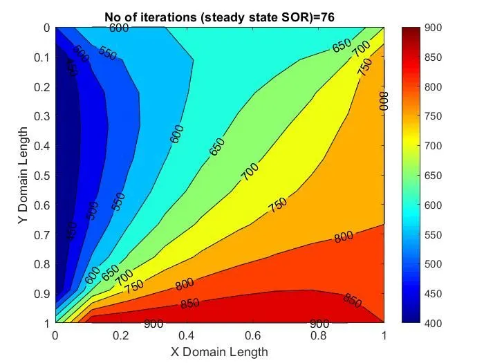
Steady state

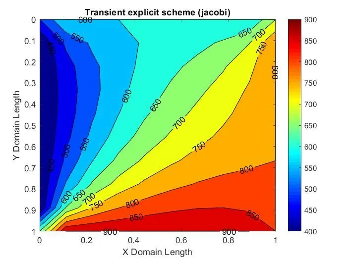
Transient state (explicit)

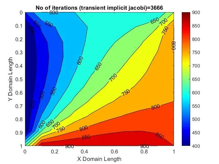
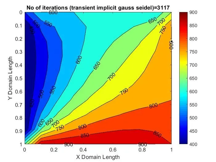
Transient state (implicit)

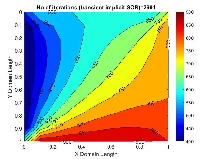
Explanation

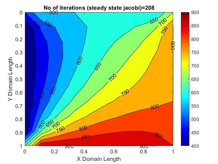
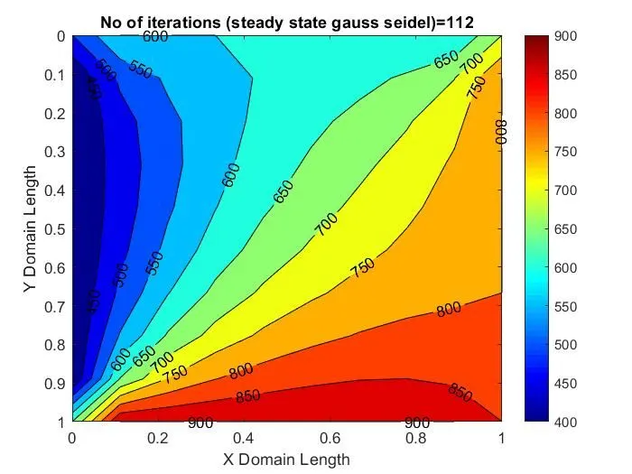
In each plot, the domain is considered as square of side length 1m. In Y direction the order is reversed (from 1 to 0) because the command set(gca,'ydir','reverse') is used. In title the method type and number of iterations are displayed. Each color in the plot denotes specific temperature value (in Kelvin).

S.no	Method	No. of iterations	Error value
1.	Steady state (Jacobi)	208	9.486811e-05
2.	Steady state (Gauss seidel)	112	9.586452e-05
3.	Steady state (Successive over relaxation)	76	8.264460e-05
4.	Transient state (Eplicit scheme, Jacobi)	-	0
5.	Transient state (Implicit scheme, Jacobi)	3666	1.250555e-12
6.	Transient state (Implicit scheme, Gauss seidel)	3117	0
7.	Transient state (Implicit scheme, Successive over relaxation)	2991	5.684342e-14

From the table, we can clearly see that the Jacobi method takes lot of iterations to converge and successive over relaxation method takes the least, whereas iterations took by gauss seidel lies between the other two methods.

Order of method based on iterations,

Jacobi>Gauss seidel>Successive over relaxation

Conclusion

• Thus in matlab, the 2D heat conduction equation is solved by using the point iterative techniques using the methods like Jacobi, Gauss-seidel, Successive over-relaxation for both implicit and explicit schemes.
• The temperature distribution plots are plotted for each methods.
• The number of iterations and error values for each methods are calculated and displayed in the above table.