Deriving 4th order approximation of a 2nd order derivative using Taylor Table method

Question

Aim

• To derive the fourth order approximations of the second-order derivative and to find out central difference, skewed right sided difference, skewed left sided difference schemes.
• To prove that the skewed schemes are fourth order accurate.
• To write a program in Matlab to evaluate the function exp(x)*cos(x) and compare with numerical approximations.
• To obtain a plot between absolute errors and the above mentioned schemes.
• To discuss the importance of skewed schemes.

Solution

Central difference scheme

Order of the accuracy(P)= no. of nodes in stencil(N)-Order of the derivative(Q)+1

`P=N-Q+1`

`4=N-2+1`

`N=5`

`Deltax^2(del^2u)/(delx^2)=af(i-2)+bf(i-1)+cf(i)+df(i+1)+ef(i+2)`

Stencil/function	f(i)	Δxf'(i)	Δx^2f''(i)	Δx^3f'''(i)	Δx^4fiv(i)	Δx^5fv(i)	Δx^6fvi(i)
af(i-2)	a	-2a	4a/2	-8a/6	16a/24	-32a/120	64a/240
bf(i-1)	b	-b	b/2	-b/6	b/24	-b/120	b/240
cf(i)	c	0	0	0	0	0	0
df(i+1)	d	d	d/2	d/6	d/24	d/120	d/240
ef(i+2)	e	2e	4e/2	8e/6	16e/24	32e/120	64e/240
Σ(stencils)	0	0	1	0	0	?	?

`a+b+c+d+e=0`

`-2a-b+0+d+2e=0`

`2a+b/2+0+d/2+2e=1`

`-(4a)/3-b/6+0+d/6+(4a)/3=0`

`(2a)/3+b/24+0+d/24+(2e)/3=0`

Skewed right sided difference scheme

No. of nodes in stencil(N)=Order of the accuracy(P)+Order of the derivative(Q)

`N=4+2`

`N=6`

`Deltax^2(del^2u)/(delx^2)=af(i)+bf(i+1)+cf(i+2)+df(i+3)+ef(i+4)+gf(i+5)`

Stencil/Function	f(i)	Δxf'(i)	Δx^2f''(i)	Δx^3f'''(i)	Δx^4fiv(i)	Δx^5fv(i)	Δx^6fvi(i)
af(i)	a	0	0	0	0	0	0
bf(i+1)	b	b	b/2	b/6	b/24	b/120	b/720
cf(i+2)	c	2c	4c/2	8c/6	16c/24	32c/120	64c/720
df(i+3)	d	3d	9d/2	27d/6	81d/24	243d/120	729d/720
ef(i+4)	e	4e	16e/2	64e/6	256e/24	1024e/120	4096e/720
gf(i+5)	g	5g	25g/2	125g/6	625g/24	3125g/120	15625g/720
Σ	0	0	1	0	0	0	?

`a+b+c+d+e+g=0`

`0+b+2c+3d+4e+5g=0`

`0+b/2+(4c)/2+(9d)/2+(16e)/2+(25g)/2=1`

`0+b/6+(8c)/6+(27d)/6+(64e)/6+(125g)/6=0`

`0+b/24+(16c)/24+(81d)/24+(256e)/24+(625g)/24=0`

`0+b/120+(32c)/120+(243d)/120+(1024e)/120+(3125g)/120=0`

Skewed left sided difference scheme

No. of nodes in stencil(N)=Order of the accuracy(P)+Order of the derivative(Q)

`N=4+2`

`N=6`

`Deltax^2(del^2u)/(delx^2)=af(i)+bf(i-1)+cf(i-2)+df(i-3)+ef(i-4)+gf(i-5)`

Stencil/Function	f(i)	Δxf'(i)	Δx^2f''(i)	Δx^3f'''(i)	Δx^4fiv(i)	Δx^5fv(i)	Δx^6fvi(i)
af(i)	a	0	0	0	0	0	0
bf(i-1)	b	-b	b/2	-b/6	b/24	-b/120	b/720
cf(i-2)	c	-2c	4c/2	-8c/6	16c/24	-32c/120	64c/720
df(i-3)	d	-3d	9d/2	-27d/6	81d/24	-243d/120	729d/720
ef(i-4)	e	-4e	16e/2	-64e/6	256e/24	-1024e/120	4096e/720
gf(i-5)	g	-5g	25g/2	-125g/6	625g/24	-3125g/120	15625g/720
Σ	0	0	1	0	0	0	?

`a+b+c+d+e+g=0`

`0-b-2c-3d-4e-5g=0`

`0+b/2+(4c)/2+(9d)/2+(16e)/2+(25g)/2=1`

`0-b/6-(8c)/6-(27d)/6-(64e)/6-(125g)/6=0`

`0+b/24+(16c)/24+(81d)/24+(256e)/24+(625g)/24=0`

`0-b/120-(32c)/120-(243d)/120-(1024e)/120-(3125g)/120=0`

Skewed schemes are fourth order accurate - proof

For skewed right sided difference scheme,

`Deltax^2(del^2u)/(delx^2)=af(i)+bf(i+1)+cf(i+2)+df(i+3)+ef(i+4)+gf(i+5)`

Since it is second order derivative, f''(i) term and f^vi(i) term exist, other coefficients of terms are equal to zero.(f^vi(i) exists because it's sum of coefficients is not known(?))

`Deltax^2(del^2u)/(delx^2)=(0+b/2+2c+(9d)/2+8e+(25g)/2)f''(i)Δx^2+(0+b/720+(4c)/45+(243d)/240+(256e)/45+(3125g)/144)f^(vi)Δx^6`

Substituting the values of a,b,c,d,e ang g values, we get,

`Deltax^2(del^2u)/(delx^2)=(1)f''(i)Δx^2+(0.11899)f^(vi)Δx^6`

Dividing both sides by `Δx^2`

`(del^2u)/(delx^2)=f''(i)+(0.11899)f^(vi)(Δx)^4`

It implies that the skewed right sided difference scheme is fourth order approximate since it has truncation error of fourth order(last term). Similarly the same will be obtained for skewed right sided difference scheme.Thus skewed schemes are fourth order accurate.

Matlab program to evaluate the second-order derivative of the analytical function exp(x)*cos(x) and comparing with the numerical approximations

Matlab code

clear all
close all
clc

%analytical function f(x)= exp(x)*cos(x)
%first order derivative f'(x)=(exp(x)*cos(x))-(exp(x)*sin(x))
%second order derivative f'(x)=-2*exp(x)*sin(x)

%Preallocation of absolute errors(Initialization)
forward_error=0;
backward_error=0;

x=pi/3;
dx=linspace(pi/400,pi/4,40);

for i=1:length(dx)

[forward_error(i), backward_error(i)]=two_approximation(x,dx(i));

end

figure(1)
loglog(dx,forward_error,'-kd','markerfacecolor','b','markersize',5)
hold on
loglog(dx,backward_error,'-ko','markerfacecolor','g','markersize',5)
hold off
legend('forward error','backward error')
xlabel('grid spacing(dx)')
ylabel('absolute error')
title('FDS and BDS error comparison')

Function code

function [error_1, error_2]=two_approximation(x,dx)

analytical_derivative=-2*exp(x)*sin(x);

%forward_differencing scheme
forward_differencing =(exp(x+dx)*cos(x+dx) - exp(x)*cos(x))/dx;

%backward_differencing scheme
backward_differencing =(exp(x)*cos(x) - exp(x-dx)*cos(x-dx))/dx;

%absolute error calculation
error_1=abs(forward_differencing - analytical_derivative);
error_2=abs(backward_differencing - analytical_derivative);

end

Explanation

• First the x value and grid spacing dx is assigned.
• For computing errors(forward and backward error) the for loop is used. For each iteration, upto length of dx, the function two_approximation is executed(where the x and dx values are passed) .
• Under the function, the second order derivative of function is computed. Then the forward differencing and backward differencing is computed.
• Then the error is computed by taking absolute difference between the forward/backward differencing value and analytical derivative value.
• When for loop ends, the errors values are computed, then using loglog command, the graph is plotted and the necessary legends, and labels are given.

Output

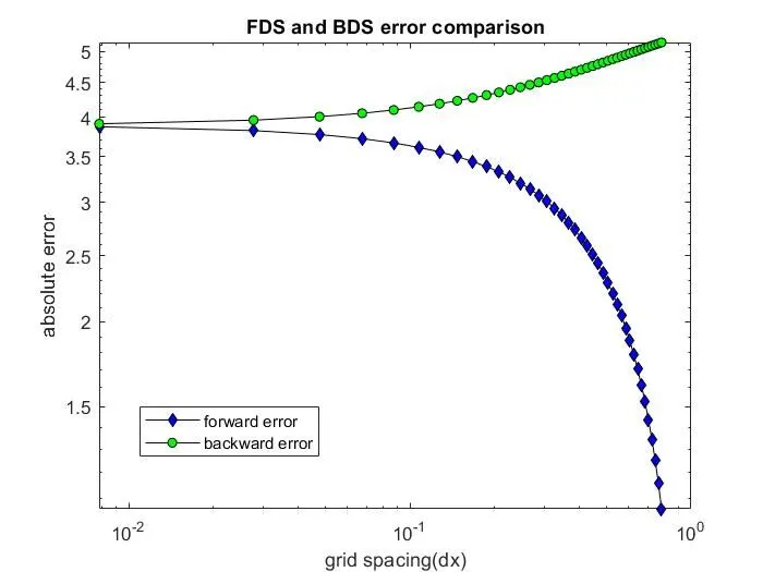
Explanation

From the graph it is seen that when the step length(grid spacing dx) increases, the forward error decreases exponentially and the backward error increases exponentialy.

Matlab program to provide a plot that compares the absolute error between the central difference and skewed schemes(left and right)

clear all
close all
clc

%Solving system of linear equations
%central differencing scheme
A=[1 1 1 1 1; -2 -1 0 1 2; 2 1/2 0 1/2 2; -4/3 -1/6 0 1/6 4/3; 2/3 1/24 0 1/24 2/3];
B=[0;0;1;0;0];
X=linsolve(A,B);

%Skewed right sided differencing scheme
C=[1 1 1 1 1 1; 
    0 1 2 3 4 5; 
    0 1/2 4/2 9/2 16/2 25/2; 
    0 1/6 8/6 27/6 64/6 125/6; 
    0 1/24 16/24 81/24 256/24 625/24; 
    0 1/120 32/120 243/120 1024/120 3125/120];
D=[0;0;1;0;0;0];
Y=linsolve(C,D);

%Skewed left sided differencing scheme
E=[1 1 1 1 1 1; 
    0 -1 -2 -3 -4 -5; 
    0 1/2 4/2 9/2 16/2 25/2; 
    0 -1/6 -8/6 -27/6 -64/6 -125/6; 
    0 1/24 16/24 81/24 256/24 625/24; 
    0 -1/120 -32/120 -243/120 -1024/120 -3125/120];
F=[0;0;1;0;0;0];
Z=linsolve(E,F);

%analytical function f(x)= exp(x)*cos(x)
%first order derivative f'(x)=(exp(x)*cos(x))-(exp(x)*sin(x))
%second order derivative f'(x)=-2*exp(x)*sin(x)

x=pi/3;
dx=linspace(pi/400,pi/4,40);

%Preallocation of absolute errors(Initialization)
skewed_left_error=0;
skewed_right_error=0;
central_difference_error=0;

for i=1:length(dx)

[central_difference_error(i), skewed_right_error(i), skewed_left_error(i)]=fourth_order_approximation(x,dx(i),X,Y,Z);

end

figure(1)
loglog(dx,central_difference_error,'-ko','markerfacecolor','b','markersize',5)
hold on
loglog(dx,skewed_right_error,'-kd','markerfacecolor','r','markersize',5)
hold on
loglog(dx,skewed_left_error,'-ks','markerfacecolor','g','markersize',5)
hold off
legend('central difference error', 'skewed right error', 'skewed left error')
xlabel('grid spacing(dx)')
ylabel('absolute error')
title('Fourth order central difference, skewed right and skewed left error comparison')

Function code

function [error_1, error_2, error_3]=fourth_order_approximation(x,dx,X,Y,Z)

analytical_derivative=-2*exp(x)*sin(x);

l=(exp(x-(5*dx)))*(cos(x-(5*dx)));
m=(exp(x-(4*dx)))*(cos(x-(4*dx)));
n=(exp(x-(3*dx)))*(cos(x-(3*dx)));
o=(exp(x-(2*dx)))*(cos(x-(2*dx)));
p=(exp(x-dx))*(cos(x-dx));
q=(exp(x))*(cos(x));
r=(exp(x+dx))*(cos(x+dx));
s=(exp(x+(2*dx)))*(cos(x+(2*dx)));
t=(exp(x+(3*dx)))*(cos(x+(3*dx)));
u=(exp(x+(4*dx)))*(cos(x+(4*dx)));
v=(exp(x+(5*dx)))*(cos(x+(5*dx)));

%fourth order second derivative central difference
central_difference=((X(1)*o)+(X(2)*p)+(X(3)*q)+(X(4)*r)+(X(5)*s))/(dx^2);

%fourth order second derivative skewed right sided difference
skewed_right_sided_difference=((Y(1)*q)+(Y(2)*r)+(Y(3)*s)+(Y(4)*t)+(Y(5)*u)+(Y(6)*v))/(dx^2);

%fourth order second derivative skewed left sided difference
skewed_left_sided_difference=((Z(1)*q)+(Z(2)*p)+(Z(3)*o)+(Z(4)*n)+(Z(5)*m)+(Z(6)*l))/(dx^2);

%absolute error calculation
error_1=abs(central_difference-analytical_derivative);
error_2=abs(skewed_right_sided_difference-analytical_derivative);
error_3=abs(skewed_left_sided_difference-analytical_derivative);

end

Explanation

• First step is to solve the linear equations for the three schemes, for example take CDS linear equations, the coefficients values of L.H.S of equation are taken in matrix A, the values of R.H.S of equation is taken in matrix B. Same procedure is followed for linear equations for skewed schemes also.
• Using linsolve command the equations are solved, coefficient values are computed and stored in variables X,Y,Z respectively.
• The x and dx values are assigned.
• For computing errors(central, skewed left, skewed right) the for loop is used. For each iteration, upto length of dx, the function fourth_order_approximation is executed(where the x,dx(i),X,Y,Z values are passed) .
• Under the function program, the second order derivative of function is computed first.
• The functions f(i-5), f(i-4),...f(i),...f(i+4),f(i+5) are assigned as l,m,...q...u,v (for simplicity) and their values are computed.
• The fourth order second derivative central difference formula is,

`(del^2u)/(delx^2)=(af(i-2)+bf(i-1)+cf(i)+df(i+1)+ef(i+2))/(Deltax^2)`

• Where a,b,c,d,e are solutions of linear equations which are computed and stored in variable X. The values f(i-2), f(i-1)...etc are computed before.
• The fourth order second derivative skewed right sided difference formula is,

`(del^2u)/(delx^2)=(af(i)+bf(i+1)+cf(i+2)+df(i+3)+ef(i+4)+gf(i+5))/(Deltax^2)`

• Where a,b,c,d,e,g are solutions of linear equations which are computed and stored in variable Y. The values f(i), f(i+1), f(i+2)...are computed before.
• The fourth order second derivative skewed left sided difference formula is,

`(del^2u)/(delx^2)=(af(i)+bf(i-1)+cf(i-2)+df(i-3)+ef(i-4)+gf(i-5))/(Deltax^2)`

• Where a,b,c,d,e,g are solutions of linear equations which are computed and stored in variable Z. The values f(i), f(i-1), f(i-2)...are computed before.
  
• Then the error is computed by taking absolute difference between the central differencing value and analytical derivative value. Same procedure is repeated for skewed schemes and their errors are computed.
• This procedure of computing the errror values for the 3 schemes for each value of dx under the function program continue upto the length of (dx), after which for loop ends.
• When for loop ends, the errors values are computed, then using loglog command, the graph is plotted and the necessary legends, and labels are given.

Verifiy that the sum of coefficients of the linear equations should be zero

>> sum(X)

ans =

   1.8041e-16

>> sum(Y)

ans =

  -2.2204e-16

>> sum(Z)

ans =

  -2.2204e-16

Since the values are close to zero, the sum of coefficients is assumed to be zero for above three cases. Hence it is verified that the solution of linear equations is nearly accurate.

Output

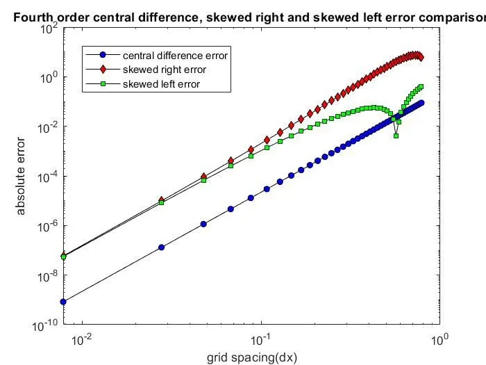
Explanation

From the graph it is seen that the error values of central difference scheme is least. Error value is highest for skewed right sided difference. Error value of skewed left sided difference is somewhat lesser than skewed right sided difference but greater than central difference scheme.i.e., central difference error < skewed left error < skewed right error. So inorder to have least error, central difference scheme can be preferred.

It can also be seen from the graph that, when value of dx decreases (i.e., moving from right to left of graph), the error values for all the 3 schemes decreases.

Actual dx value taken: dx=linspace(pi/400,pi/4,40).

So let us further decrease the value of dx and see how graph looks like after running the program. So let's take, dx=linspace(pi/400000,pi/4,40).

Output (wrong)

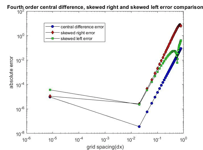
So when dx value is reduced further, the error values for the 3 schemes instead of decreasing (i.e., moving from right to left of graph) ,the error values start to increase. This is because of round-off error. So inorder to keep away from this error, it is advised to keep the step length (grid spacing) dx in optimum value (not much less than 10^-3).

The above graph is plotted just to show the effect of round-off error when having very much smaller dx value. This graph is absolutely wrong because it cannot be used for comparing the errors of three schemes.

Importance of skewed schemes

In all cases, central difference scheme cannot be used. Skewed schemes are used when the points are available only on the one side of the grid. Inorder to calculate the higher order (4th order) approximation value for the corner node, skewed schemes can be used because central differencing scheme requires points on both the sides(before and after) which is not possible for corner node.

Conclusion

• Fourth order second-order derivative central difference, skewed right sided difference, skewed left sided difference schemes are derived using taylor table method.
• Skewed schemes are fourth order accurate- hence proved.
• Using matlab, the function exp(x)*cos(x) is evaluated for its second order derivative and plot is obtained representing absolute errors of FDS and BDS (forward/backward difference schemes) with respect to dx .
• Using matlab, the function exp(x)*cos(x) is evaluated for its second order derivative and plot is obtained representing absolute errors of CDS (central difference schemes) and skewed schemes with respect to dx.
• Round-off error comes to play due to very less value of dx, is discussed.
• Importance of skewed schemes is discussed.