Understanding the stability analysis in linear systems using MATLAB

GIVEN: Coefficient Matrix, A=[5 1 2 ; -3 9 4; 1 2 -7]
Solution Matrix, X=[x1;x2;x3]
Residual Matrix, B=[10 -14 33]

OBJECTIVES:

• To solve the system of matrices using Jacobi, Gauss-seidel, and SOR methods.
• To compute the Iteration Matrix for the above-mentioned methods by suitable matrix decomposition techniques.
• To calculate the Eigenvalues of the Iteration matrix.
• To calculate the Spectral radius of the Iteration matrix.
• To explain the concept of Eigenvalue & Spectral radius of the matrix and its effect on the convergence rate of the solution.
• To derive a relationship between Diagonal dominance and spectral radius.

THEORY:

Discretizing the governing equations of fluid flow and heat transfer results in a system of linear algebraic equations which needs to be solved. The complexity and size of the set of equations depend on the - dimensionality of the problem, the number of grid nodes, and the discretization practice. There are two families of solution techniques for linear algebraic equations: direct methods and indirect or iterative methods. Simple examples of direct methods are Cramer’s rule matrix inversion and Gaussian elimination. The number of operations to the solution of a system of `N`equations with `N` unknowns by means of a direct method can be determined beforehand and is of the order of `N^3`. The simultaneous storage of all `N^3` coefficients of the set of equations in core memory is required.

Iterative methods are based on the repeated application of a relatively simple algorithm leading to eventual convergence after a – sometimes large – number of repetitions. Well-known examples are the Jacobi and Gauss-Seidel point-iterative methods. The total number of operations, typically of the order of `N` per iteration cycle, cannot be predicted in advance. Stronger still, it is not possible to guarantee convergence unless the system of equations satisfies fairly exacting criteria. The main advantage of iterative solution methods is that only non-zero coefficients of the equations need to be stored in core memory.

The Jacobi and Gauss-Seidel methods are general-purpose point-iterative algorithms that are easily implementable, but their convergence rate can be slow when the system of equations is large. They were not initially considered suitable for general-purpose CFD procedures. However, more recently multigrid acceleration techniques have been developed that have improved the convergence rates of iterative solvers to such an extent that they are now the method of choice in commercial CFD codes.

1. Point-iterative methods

Point-iterative techniques are introduced by means of a simple example. Consider a set of three equations and three unknowns:

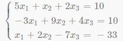
In iterative methods we rearrange the first equation to place x1 on the left-hand side, the second equation to get x2 on the left-hand side, and so on. This yields

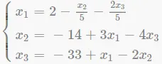
We see that unknowns ``and `` appear on both sides of ``.The system of equations can be solved iteratively by substituting a set of guessed initial values for x1, x2, and x3 on the right-hand side. This allows us to calculate new values of the unknowns on the left-hand side of ``. The next move is to substitute the new values back into the right-hand side and evaluate the unknowns on the left-hand side again, which are, if the procedure converges, closer to the true solution of the system of equations. This process is repeated until there is no more change in the solution.

1.1. Jacobi

The generalized iteration equation for the Jaocbi method is:

`x_i^((k)) = sum_(j=1,j!=1)^n((-a_(ij))/a_(ii))x_j^((k-1))+b_i/a_(ii) (i=1,2,....,n)`

In matrix form this equation can be written as follows:

`x^((k)) = T.x^((k-1)) + C` where `T` = iteration matrix, `C` = constant vector

1.2. Gauss-Seidel

The generalized iteration equation for the Gauss-Seidel method is:

`x_i^((k)) = sum_(j=1)^(i-1)((-a_(ij))/a_(ii))x_j^((k))+ sum_(j=i+1)^(n)((-a_(ij))/a_(ii))x_j^((k-1)) + b_i/a_(ii) (i=1,2,....,n)`

In matrix form we have,

`x^((k)) = T_1.x^((k)) + T_2.x^((k-1)) + C`

1.3. Successive Over-Relaxation (SOR)

The convergence rate of the Jacobi and Gauss-Seidel methods depends on the properties of the iteration matrix. It has been found that these can be improved by the introduction of a so-called relaxation parameter `omega`.

`x^((k)) = (1-omega).x^((k-1)) + omega.x_(GS)`

When we choose `0 < omega < 1` the procedure is an under-relaxation method, whereas `omega> 1` is called over-relaxation.

There exist special classes of matrices for which it is possible to state some convergence results. One condition for the iteration process to be convergent is that the matrix must be diagonally dominant.

2. Foundations of Matrix Analysis

Let `m` and `n` be two positive integers. We call a matrix having `m` rows and `n` columns, or a matrix `m*n` or a matrix `(m,n)` with elements in `K`, a set of `mn` scalars `a_(ij) in K`, with `i=1,...,m` and `j=1,...,n` represented in the following rectangular array:

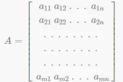
When `K = R` or `K = C` we shall respectively write `A in R^ (mxxn)` or `A in C^ (mxxn)`.The index `i` is called row index, while `j` is the column index. The set `(a_(i1),a_(i2),...,a_(i n))` is called the `i - th` row of `A`; likewise, `(a_(1j),a_(2j),...,a_(mj))` is the `j - th` column of `A`.
If `n=m`, the matrix is called squared or has order `n`, and the set of the entries `(a_(11),a_(22),...,a_(n n))` is called it's main diagonal. A matrix having one row or one column is called a row vector or column vector respectively.

2.1. Diagonally Dominant

A matrix `A in R^(nxxn)` is called diagonally dominant by rows if

`abs(a_(ii))>= sum_(j=1,j!=i)^n abs(a_(ij)), {i=1,....,n}`

while it is called diagonally dominant by columns if

`abs(a_(ii))>= sum_(j=1,j!=i)^n abs(a_(ji)), {i=1,....,n}`

If the inequalities above hold in a strict sense, `A` is called strictly diagonally dominant (by rows or by columns, respectively). If `A` is a strictly diagonally dominant matrix, the Jacobi and Gauss-Seidel methods are convergent.

2.2. Eigenvalues & Spectral Radius

Let `A` be a square matrix of order `n` with real or complex entries; the number `lambdainC`is called an eigen value of `A` if there exists a nonnull vector `x in C^n`such that `Ax = lambdax`. The vector `x` is the eigenvector associated with the eigenvalue `lambda` and the set of the eigenvalues of `A` is called the spectrum of `A`, denoted by `sigma(A)`

The number `lambda` is the solution of the characteristic equation

`P_A(lambda) = det(A-lambdaI) = 0`, where `P_A(lambda)` is the characteristic polynomial.

The maximum module of the eigenvalues of `A` is called the spectral radius of `A` and is denoted by

`rho(A) = max_(lambdainA) abs(lambda)`

2.3 LDU Decomposition

LDU decomposition can be applied to different solvers to perform convergence studies.

`A=[[5,1,2],[-3,9,4],[1,2,-7]]`, `b=[[10],[-14],[-33]]`, `x=[[x],[x],[x]]`

`U=[[0,1,2],[0,0,4],[0,0,0]]`, `D=[[5,0,0],[0,9,0],[0,0,-7]]`, `L=[[0,0,0],[-3,0,0],[1,2,0]]`

A general iterative function would be of the form:

`x^((k)) = T.x^((k-1)) + C`

2.3.1 Jacobi

We know that a general system linear equation takes the form `A.x=b`. Expanding `A` as `L+D+U` and taking `L+U` to the other side, and simplifying, we get,

`x^((k)) = -D^(-1).(L+U).x^((k-1))+D^(-1).b`

where, `T_(iter)^(Jacobi) = -D^(-1).(L+U)` and

`C = D^(-1).b`

2.3.2 Gauss-Seidel

Similarly, for Gauss-Seidel we get,

`x^((k)) = (L+D)^(-1).x^((k-1))+(L+D)^(-1).b`

where, `T_(iter)^(SOR) = I-omega((L+D)^(-1).U+I)`, and

`C = (L+D)^(-1).b`

2.3.3 SOR

`x^((k)) = omega.(L+D)^(-1).b+(I-omega((L+D)^(-1).U+I))x^((k-1))`

where, `T_(iter)^(SOR) = I-omega((L+D)^(-1).U+I)`, and

`C = omega.(L+D)^(-1).b`

CODE:

1. Main Code

clear all
close all
clc

% Initialization
A = [5 1 2; -3 9 4; 1 2 -7];
B = [10; -14; 33];
% matrix decomposition)
L = [0 0 0; -3 0 0; 1 2 0];
U = [0 1 2; 0 0 4; 0 0 0];
D =diag(diag(A));
I = eye(3);
mag_factor = linspace(0.2,1.5,20);
omega = 0.95;

for i = 1:length(mag_factor)
    Dm = mag_factor(i)*D;
    
    % Computing the iteration matrix
    Tjac = -inv(Dm)*(L+U); 
    Tgs = -inv(L+Dm)*U;
    T_SOR = I-omega*((inv(L+Dm)*U)+I);
    
    % Computing the eigen values
    e_jac = roots(poly(Tjac));
    e_gs = roots(poly(Tgs));
    e_SOR = roots(poly(T_SOR));
    
    % Computing the spectral radius
    rho_jac(i) = max(abs(e_jac));
    rho_GS(i) = max(abs(e_gs));
    rho_SOR(i) = max(abs(e_SOR));
    
    % Calling the iterative solvers
    [jac_iter(i), x_jac(i,:),jac_error] = jac(Dm,L,U,B);
    [GS_iter(i), x_GS(i,:), GS_error] = GS(Dm,L,U,B);
    [SOR_iter(i), x_SOR(i,:), SOR_error] = SOR(Dm,L,U,B,omega);
end

% Errors
fprintf('Error calculated using Jacobi method= %d',jac_error)
fprintf('nError calculated using Gauss seidel method= %d',GS_error)
fprintf('nError calculated using SOR method= %d',SOR_error)

% Plotting
% 1.Jacobi
figure(1)
subplot(2,1,1)
plot(rho_jac,jac_iter,'-x','markerfacecolor','r','markeredgecolor','r','color','k','linewidth',1.5);
title('Jacobi Method ');
xlabel('Spectral Radius');
ylabel('No.of iterations');
axis([0.2 1.6 0 inf])
grid on
subplot(2,1,2)
plot(rho_jac,mag_factor, '-x','markerfacecolor','r','markeredgecolor','r','color','k','linewidth',1.5);
ylabel('Magnification Factor');
xlabel('Spectral Radius');
yticks(0:.5:1.5);
axis([0.2 1.6 0 inf])
grid on

% 2.Gauss-Seidel
figure(2)
subplot(2,1,1)
plot(rho_GS,GS_iter, '-x','markerfacecolor','r','markeredgecolor','r','color','k','linewidth',1.5);
title('GS Method');
xlabel('Spectral Radius');
ylabel('No.of iterations');
axis([0.2 1.6 0 inf])
grid on
subplot(2,1,2)
plot(rho_GS,mag_factor,'-x','markerfacecolor','r','markeredgecolor','r','color','k', 'linewidth',1.5);
ylabel('Magnification Factor');
xlabel('Spectral Radius');
yticks(0:.5:1.5);
axis([0.2 1.6 0 inf])
grid on


% 3.SOR
figure(3)
subplot(2,1,1)
plot(rho_SOR,SOR_iter, '-x','markerfacecolor','r','markeredgecolor','r','color','k','linewidth',1.5);
title('SOR Method');
xlabel('Spectral Radius');
ylabel('No.of iterations');
axis([0.2 1.6 0 inf])
grid on
subplot(2,1,2)
plot(rho_SOR,mag_factor,'-x','markerfacecolor','r','markeredgecolor','r','color','k', 'linewidth',1.5);
ylabel('Magnification Factor');
xlabel('Spectral Radius');
yticks(0:.5:1.5);
axis([0.2 1.6 0 inf])
grid on

% 4.Magnification factors vs Spectral radii
figure(4)
Magnification_factors = mag_factor;
Spectral_Radii = zeros(20,3);
Spectral_Radii = transpose([rho_jac;rho_GS;rho_SOR]);
plot(Magnification_factors,Spectral_Radii,'-x','markeredgecolor','k','linewidth',1.5);
legend('Spectral Radii(Jac.)','Spectral Radii(GS)','Spectral Radii(SOR)');
xlabel('Magnification Factor');
xticks(0:0.1:1.6)
ylabel('Spectral Radii');
yticks(0:1:12);
grid on

2. Functions

Jacobi

function[jac_iter, x_jac,jac_error ] = jac(Dm,L,U,B)

% initialization
x = zeros(3,1); 
xold=x;
jac_error = 9e9;
tol = 1e-4;
jac_iter= 0;

    while(jac_error>tol)
        x = inv(Dm)*(B-((L+U)*xold));
        jac_error = max(abs(x-xold));
        xold = x;
        jac_iter = jac_iter + 1;
    end
    x_jac = x;
end

Gauss-Seidel

function[GS_iter, x_GS, GS_error] = GS(Dm,L,U,B)

% initialization
x = zeros(3,1);
xold = x;
GS_error = 9e9;
tol = 1e-4;
GS_iter = 0;

    while(GS_error>tol)
        x = inv(L+Dm)*(B-U*xold);
        GS_error = max(abs(x-xold));
        xold = x;
        GS_iter = GS_iter + 1;
    end
    x_GS = x;
end

SOR

function[SOR_iter, x_SOR, SOR_error] = SOR(Dm,L,U,B,omega)

% initialization
x = zeros(3,1);
xold = x;
SOR_iter = 0;
SOR_error = 9e9; 
tol = 1e-4;

    while(SOR_error>tol)
        x=(inv(omega*L+Dm))*(-(omega*U+(omega-1)*Dm))*xold+(inv(omega*L+Dm))*(omega*B);
        SOR_error = max(abs(x - xold));
        xold = x;
        SOR_iter = SOR_iter + 1;
    end
    x_SOR = x;
end

RESULTS & DISCUSSION:

In`fig.(1)`, we can see that our final errors for all the three iterative solvers are below our tolerance `1e-4`.

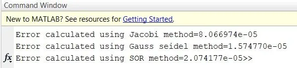
`fig(1)`: Errors at the end of iterations

From the table in `fig.(2)` and graphs in `fig.(3)`, we clearly witness the relationship between spectral radius and magnification factors (diagonal dominance). As the value of magnification factors increases, the value of spectral radius decreases i.e. spectral radius is inversely proportional to the magnification factor. We also observe that for magnification factor values above `0.5`(approx.), the spectral radius values tend to fall below `1`, which is an important factor for convergence as we shall observe in the upcoming results.

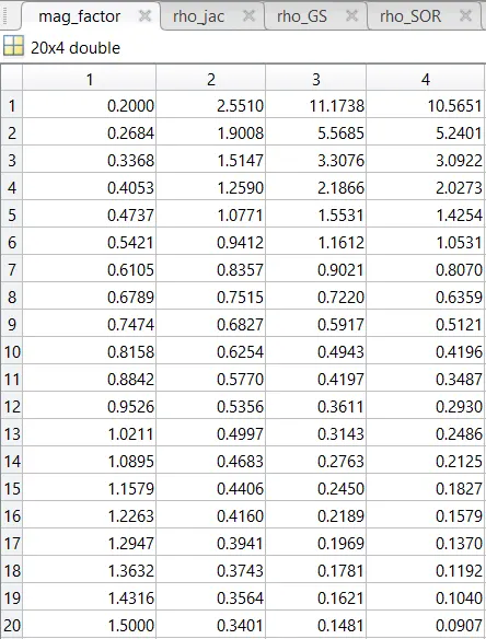
`fig.(2)`: Magnification factors and the Spectral Radii

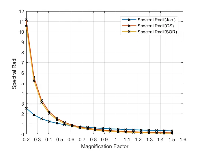
`fig.(3)`: Behaviour of spectral radii for different magnification factors

From `fig.(4)`, `fig.(5)`, and `fig.(6)`, we can conclude that as the spectral radius value approaches and is more than `1`, the solution becomes unstable. The number of iterations increases and the solution becomes divergent. In this case, Matlab terminates the iteration when it sees the spectral radius is too large and the solution is diverging. The SOR method is more or less rapidly convergent, depending on the choice of the relaxation parameter `omega`.

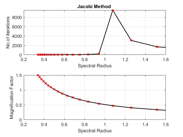
`fig.(4)`: Effect of spectral radius on convergence for the Jacobi solver

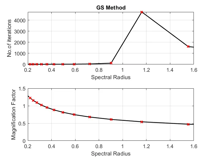
`fig.(5)`: Effect of spectral radius on convergence for the Gauss-Seidel solver

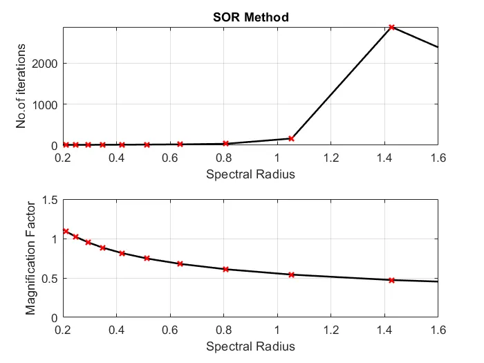
`fig.(6)`: Effect of spectral radius on convergence for the SOR solver

These iterative methods are general-purpose point-iterative algorithms that are easily implementable, but their convergence rate can be slow when the system of equations is large. More recently multigrid acceleration techniques have been developed that have improved the convergence rates of iterative solvers to such an extent that they are now the method of choice in commercial CFD codes.