Transient simulation of an incompressible, laminar, viscous flow through a backward-facing step in OpenFOAM
OBJECTIVE:
- To set-up and perform the simulation in OpemFOAM.
- To measure the velocity profile at 0.085 m from the inlet of the geometry.
- To explain why the Grading/Growth factor is essential for meshing.
INTRODUCTION:
OpenFOAM is a free, open-source CFD software that is a three-dimensional CFD tool, based on the finite volume method (FVM).
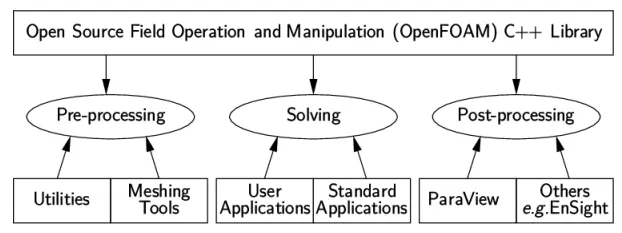
Fig.1: Overview of an OpenFOAM structure
An OpenFOAM test case is a directory that generally contains at least three folders. Fig.2 shows the innards of the cavity test case folder, which consists of the following three sub-folders:
- The 'system' directory contains at least three files with information about the case setup, the schemes to be used, and the various solution parameters. These files are: (i) controlDict which is concerned with the general control parameters of the test case such as the simulation starting and ending times, the time step to be used, and required parameters for data output; (ii) fvSchemes in which the discretization schemes used in the simulation are defined; (iii) fvSolution that contains information related to the solution algorithms and relaxations used during simulation.
- The 'constant' directory contains information about relevant physical properties, e.g., transportProperties, and the data describing the grid system used within a folder denoted by polyMesh.
- The ‘time’ directories contain initialization and boundary condition information about the fields used in the test case. It is also the folder where results for various time steps are stored. The name of each sub-folder refers to the time at which the simulation was performed. For example, in the cavity tutorial shown in Fig. 2, the velocity field U and pressure field p are initialized from files in the ‘0’ folder 0/U and 0/p, respectively.
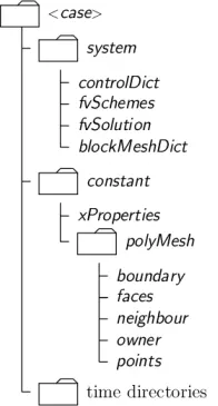
Fig.2: The cavity OpenFOAM case
The solver for this simulation was chosen to be icoFoam, chosen from this guide - 'standard solvers'.
1. Pre-processing
Cases are set up in OpenFOAM by editing case files. As a first step, the cavity case directory was copied from the tutorial folder to the run directory. The contents of this folder was explained above.
1.1 Mesh Generation
OpenFOAM always operates in a 3-dimensional Cartesian coordinate system and all geometries are generated in 3 dimensions. OpenFOAM solves the case in 3 dimensions by default but can be instructed to solve in 2 dimensions by specifying a ‘special’ empty boundary condition on boundaries normal to the (3rd) dimension for which no solution is required (as done in our case). The domain specifications are provided in the following figure:
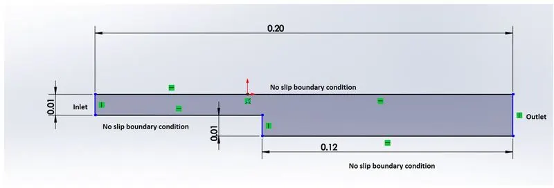
Fig.3: Geometry and boundary conditions
Mesh specification-
- Number of cells along the x direction (longer dimension) = 200
- Number of cells along the longer y direction = 20
The mesh generator supplied with OpenFOAM, blockMesh, generates meshes from a description specified in the input dictionary, blockMeshDict, located in the system directory for a given case. The principle behind blockMesh is to decompose the domain geometry into a set of 1 or more three dimensional, hexahedral blocks. Edges of the blocks can be straight lines, arcs, or splines. Each block of the geometry is defined by 8 vertices, one at each corner of a hexahedron. The vertices are written in a list so that each vertex can be accessed using its label, remembering that OpenFOAM always uses the C++ convention that the first element of the list has the label ‘0’. The file first contains header information in the form of a banner (lines 1-7), then file information contained in a FoamFile sub-dictionary, delimited by curly braces ({…}). The file first specifies coordinates of the block vertices; it then defines the blocks (here, 5) from the vertex labels and the number of cells within it; and finally, it defines the boundary patches.
1.1.1 Importance of grading/growth factor in meshing
The error in any solution will be more pronounced in regions where the form of the true solution differs widely from the form assumed in the chosen numerical schemes. For example, a numerical scheme based on linear variations of variables over cells can only generate an exact solution if the true solution is itself linear in form. The error is largest in regions where the true solution deviates greatest from linear form, i.e. where the change in gradient is largest. Error decreases with cell size. In this case, large variations in velocity can be expected near the step wall and so the mesh will be graded to be smaller in this region. By using the same number of cells, greater accuracy can be achieved without a significant increase in computational cost.
BlockMeshDict file for Case 1: No grading factor (i.e., GF = 1)
/*--------------------------------*- C++ -*----------------------------------*
  =========                 |
  \      /  F ield         | OpenFOAM: The Open Source CFD Toolbox
   \    /   O peration     | Website:  https://openfoam.org
    \  /    A nd           | Version:  9
     \/     M anipulation  |
*---------------------------------------------------------------------------*/
FoamFile
{
    format      ascii;
    class       dictionary;
    object      blockMeshDict;
}
// * * * * * * * * * * * * * * * * * * * * * * * * * * * * * * * * * * * * * //

convertToMeters 1;

vertices
(
    //vertices from point 0 to 10
    (0 0 0)
    (0.08 0 0)
    (0.08 0.005 0)
    (0 0.005 0)
    (0.08 0.01 0)
    (0 0.01 0)
    (0.2 0.01 0)
    (0.2 0.005 0)
    (0.2 0 0)
    (0.2 -0.01 0)
    (0.08 -0.01 0)

    //vertices from point 11 to 21
    (0 0 0.1)
    (0.08 0 0.1)
    (0.08 0.005 0.1)
    (0 0.005 0.1)
    (0.08 0.01 0.1)
    (0 0.01 0.1)
    (0.2 0.01 0.1)
    (0.2 0.005 0.1)
    (0.2 0 0.1)
    (0.2 -0.01 0.1)
    (0.08 -0.01 0.1)
);

blocks
(
    // Block 1
    // hex=shape identifier
    hex (0 1 2 3 11 12 13 14) (80 5 1) simpleGrading (1 1 1)
    // Block 2
    hex (3 2 4 5 14 13 15 16) (80 5 1) simpleGrading (1 1 1)
    // Block 3
    hex (2 7 6 4 13 18 17 15) (120 5 1) simpleGrading (1 1 1)
    // Block 4
    hex (1 8 7 2 12 19 18 13) (120 5 1) simpleGrading (1 1 1)
    // Block 5
    hex (10 9 8 1 21 20 19 12) (120 10 1) simpleGrading (1 1 1)

);

edges
(
);

boundary
(
    inlet
    {
        type patch;
        faces
        (
            (11 14 3 0)
            (14 16 5 3)
        );
    }
    outlet
    {
        type patch;
        faces
        (
            (20 9 8 19)
            (19 8 7 18)
            (18 7 6 17)
        );
    }

    noslipwalls
    {
    	type wall;
    	faces
    	(
    	    //top
    	    (16 15 4 5)
    	    (15 17 6 4)
    	    //stepside
    	    (21 12 1 10)
    	    //bottom of1
    	    (11 0 1 12)
    	    //bottom of5
    	    (21 10 9 20)
    	);
    }
    frontandback
    {
        type empty; //OF wont solve anything for this
        faces
        (
            //back
            (9 10 1 8)
            (8 1 2 7)
            (7 2 4 6)
            (1 0 3 2)
            (2 3 5 4)
            //front
            (20 19 12 21)
            (19 18 13 12)
            (18 17 15 13)
            (13 15 16 14)
            (12 13 14 11)
        );
    }
);
mergePatchPairs
(
);

// ************************************************************************* // 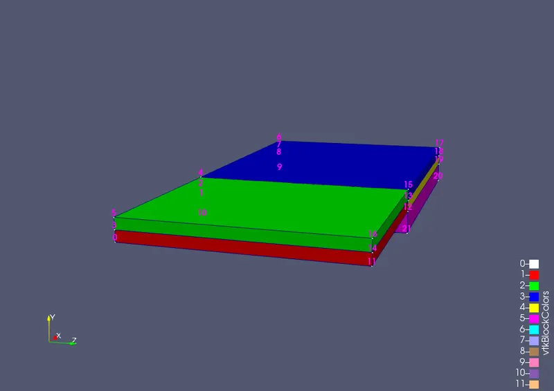
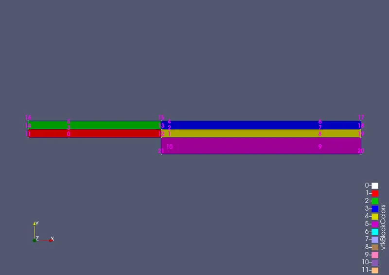
Fig. 4: 21 Vertices and 5 blocks
BlockMeshDict file for Case 2: Grading Factor, GF = 0.2
blocks
(
    // Block 1
    // hex=shape identifier
    hex (0 1 2 3 11 12 13 14) (80 5 1) simpleGrading (0.2 5 1)
    // Block 2
    hex (3 2 4 5 14 13 15 16) (80 5 1) simpleGrading (0.2 0.2 1)
    // Block 3
    hex (2 7 6 4 13 18 17 15) (120 5 1) simpleGrading (5 0.2 1)
    // Block 4
    hex (1 8 7 2 12 19 18 13) (120 5 1) simpleGrading (5 5 1)
    // Block 5
    hex (10 9 8 1 21 20 19 12) (120 10 1) simpleGrading (5 5 1)

);
1.2 Boundary and initial conditions
We can review the initial fields set up for this example after the mesh generation is finished. The initial field data is kept in a '0' sub-directory because the case is configured to begin at time = 0. The 0 sub-directory contains 2 files, p and U, one for each of the pressure (p) and velocity (U) fields whose initial values and boundary conditions must be set.
Let us examine the pressure file p:
dimensions      [0 2 -2 0 0 0 0];

internalField   uniform 0;

boundaryField
{
    inlet
    {
        type            zeroGradient;
    }

    outlet
    {
        type            fixedValue;
        value 		 uniform 0;
    }

    noslipwalls
    {
    	type 		 zeroGradient;
    }

    frontandback
    {
        type            empty;
    }
}

// ************************************************************************* //
There are 3 principal entries in field data files:
- dimensions
- - specifies the dimensions of the field, here kinematic pressure, i.e. `m^2s^2`;
internalField
- the internal field data which can be uniform, described by a single value; or nonuniform, where all the values of the field must be specified;
boundaryField
- the boundary field data that includes boundary conditions and data for all the boundary patches.
For this case, the boundary consists of
- inlet - zeroGradient, meaning 'the normal gradient of pressure is zero'
- outlet - fixedValue;
- noslipwalls - zeroGradient; and
- frontandback (represents the front and back planes of the 2D case) - empty
In this case, the initial fields are set to be uniform. The pressure is kinematic, and as an incompressible case, its absolute value is not relevant, so is set to uniform 0 for convenience.
We can similarly examine the velocity field in the 0/U file. The dimensions are those expected for velocity, the internal field is initialized as uniform zero, which in the case of velocity must be expressed by 3 vector components, i.e. uniform (0 0 0). The boundary field for velocity requires the same boundary condition for the frontandback patch. The flow velocity at the inlet is 0.1 m/s in the `x`-direction so requires a fixedValue condition with the value of uniform (0.1 0 0).
Velocity file U:
dimensions      [0 1 -1 0 0 0 0];

internalField   uniform (0 0 0);

boundaryField
{
    inlet
    {
        type            fixedValue;
        value           uniform (0.1 0 0);
    }

    outlet
    {
        type            zeroGradient;
    }

    noslipwalls
    {
        type		 noSlip;
    }

    frontandback
    {
        type            empty;
    }
}

// ************************************************************************* //
1.3 Physical properties
The physical properties are stored in dictionary files in the 'constant' directory. For an icoFoam case, the only property that must be specified is the kinematic viscosity `nu`. This case will be run with a Reynolds number of 100, where the Reynolds number is defined as:
`Re=(UL)/nu`
where U and L are the characteristic velocity and length (in this case, step length) of the mean flow and `nu` is the kinematic viscosity. Here `U`=0.1m/s, `L`=0.1m, so that for `Re`=100, `nu` = 1e-5 `m^2s^(-1)`. Therefore, the following information is the proper file entry for kinematic viscosity:
nu              [0 2 -1 0 0 0 0] 1e-5;


// ************************************************************************* //
1.4 Control
Input data relating to the control of time and reading and writing of the solution data are read in from the controlDict dictionary (located in the system directory). To achieve temporal accuracy and numerical stability when running icoFoam, a Courant number `C` of less than 1 is required. The flow velocity varies across the domain and we must ensure `C`<1 everywhere. We, therefore, choose `delt` based on the worst case: the maximum `C`. The Courant number is defined for one cell as:
`C = (U.delt)/(delx)`
where `U` is the magnitude of the velocity through that cell, `delt` is the time step and `delx` is the cell size in the direction of the velocity.
The cell size is:
`delx = L/n= 0.2/200 = 0.001 m`
Therefore, `delt = (C.delx)/U = (1 xx 0.001)/0.1= 0.01 s`
As the simulation progresses we wish to write results at certain intervals of time that we can later view with a post-processing package. The writeControl keyword presents several options for setting the time at which the results are written; here we select the runTime option which specifies that results are written every `n`th time step where the value `n` is specified under the writeInterval keyword, in this case, 0.2.
ControlDict file-
application     icoFoam;

startFrom       startTime;

startTime       0;

stopAt          endTime;

endTime         5;

deltaT          0.001;

writeControl    runTime;

writeInterval   0.2;

purgeWrite      0;

writeFormat     ascii;

writePrecision  6;

writeCompression off;

timeFormat      general;

timePrecision   6;

runTimeModifiable true;


// ************************************************************************* //
fvSolutions and fvSchemes were not changed for this simulation.
2. Viewing the mesh
The mesh is viewed in ParaView, the post-processing tool supplied with OpenFOAM. The ParaView post-processing is conveniently launched on OpenFOAM case data by executing the paraFoam script from within the case directory.
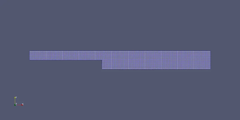
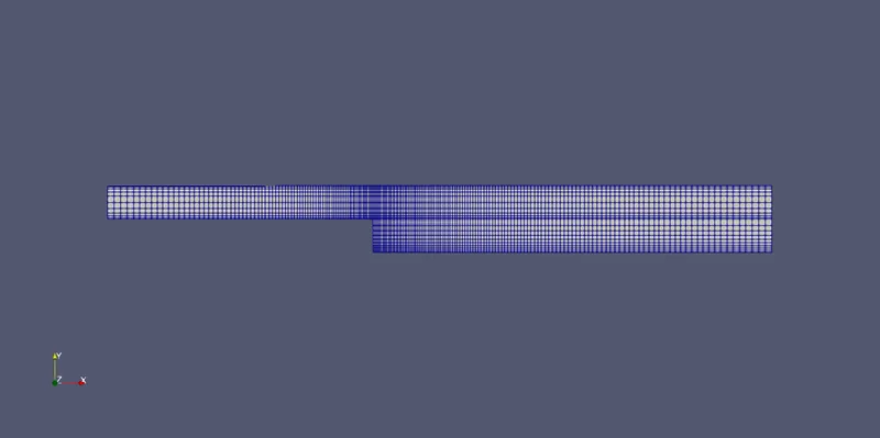
Fig.5: Mesh with grading factor GF = 1 (left); and GF = 0.2 (right)
3. Solving
The icoFoam solver is executed in the case directory. The progress of the job is written on the terminal window. It tells the user the current time, maximum Courant number, initial, and final residuals for all fields.
Time = 4.997

Courant Number mean: 0.0657407 max: 0.151959
smoothSolver:  Solving for Ux, Initial residual = 6.49168e-06, Final residual = 6.49168e-06, No Iterations 0
smoothSolver:  Solving for Uy, Initial residual = 8.8219e-06, Final residual = 8.8219e-06, No Iterations 0
DICPCG:  Solving for p, Initial residual = 4.00913e-06, Final residual = 8.63508e-07, No Iterations 14
time step continuity errors : sum local = 2.56151e-11, global = 1.63297e-12, cumulative = 4.1013e-07
DICPCG:  Solving for p, Initial residual = 3.54139e-06, Final residual = 8.79145e-07, No Iterations 4
time step continuity errors : sum local = 2.60789e-11, global = 1.78855e-12, cumulative = 4.10131e-07
ExecutionTime = 34.4 s  ClockTime = 35 s

Time = 4.998

Courant Number mean: 0.0657407 max: 0.151959
smoothSolver:  Solving for Ux, Initial residual = 6.48613e-06, Final residual = 6.48613e-06, No Iterations 0
smoothSolver:  Solving for Uy, Initial residual = 8.81512e-06, Final residual = 8.81512e-06, No Iterations 0
DICPCG:  Solving for p, Initial residual = 3.86544e-06, Final residual = 9.45799e-07, No Iterations 16
time step continuity errors : sum local = 2.80561e-11, global = 3.15906e-12, cumulative = 4.10134e-07
DICPCG:  Solving for p, Initial residual = 3.66224e-06, Final residual = 9.85998e-07, No Iterations 4
time step continuity errors : sum local = 2.92485e-11, global = 3.30138e-12, cumulative = 4.10138e-07
ExecutionTime = 34.4 s  ClockTime = 35 s

Time = 4.999

Courant Number mean: 0.0657406 max: 0.151959
smoothSolver:  Solving for Ux, Initial residual = 6.48019e-06, Final residual = 6.48019e-06, No Iterations 0
smoothSolver:  Solving for Uy, Initial residual = 8.80467e-06, Final residual = 8.80467e-06, No Iterations 0
DICPCG:  Solving for p, Initial residual = 4.01073e-06, Final residual = 8.44305e-07, No Iterations 7
time step continuity errors : sum local = 2.50453e-11, global = 4.17093e-12, cumulative = 4.10142e-07
DICPCG:  Solving for p, Initial residual = 3.56887e-06, Final residual = 9.18168e-07, No Iterations 8
time step continuity errors : sum local = 2.72363e-11, global = 4.1995e-12, cumulative = 4.10146e-07
ExecutionTime = 34.4 s  ClockTime = 35 s

Time = 5

Courant Number mean: 0.0657406 max: 0.151959
smoothSolver:  Solving for Ux, Initial residual = 6.47476e-06, Final residual = 6.47476e-06, No Iterations 0
smoothSolver:  Solving for Uy, Initial residual = 8.79019e-06, Final residual = 8.79019e-06, No Iterations 0
DICPCG:  Solving for p, Initial residual = 4.4336e-06, Final residual = 9.35602e-07, No Iterations 15
time step continuity errors : sum local = 2.77534e-11, global = 6.37214e-12, cumulative = 4.10152e-07
DICPCG:  Solving for p, Initial residual = 3.66225e-06, Final residual = 9.88376e-07, No Iterations 4
time step continuity errors : sum local = 2.93188e-11, global = 6.8531e-12, cumulative = 4.10159e-07
ExecutionTime = 34.41 s  ClockTime = 35 s

End
4. Post-Processing
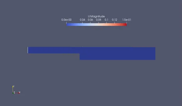
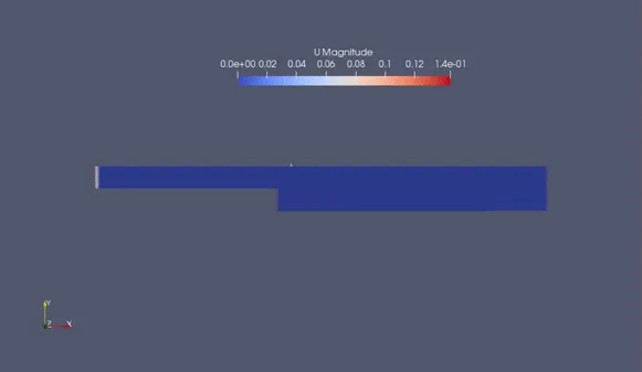
Animation: Velocity in the domain: GF = 1 (left); and GF = 0.2 (right)
Discussion:
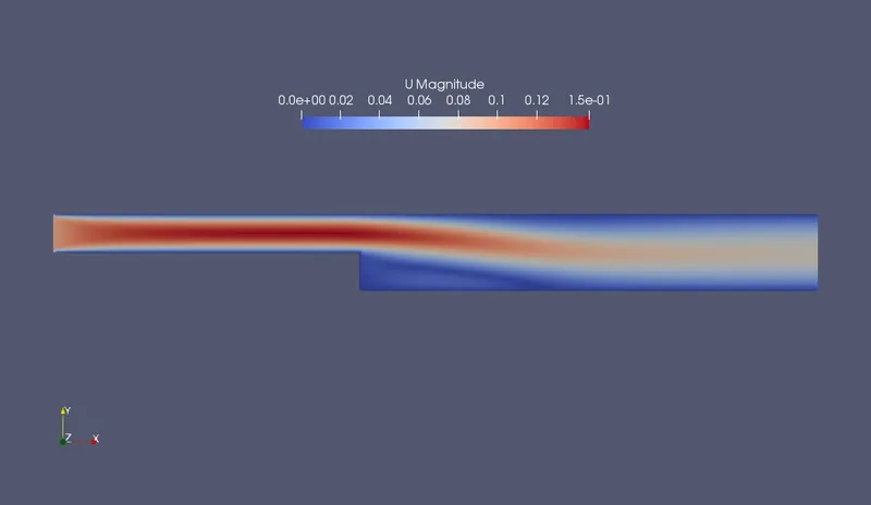
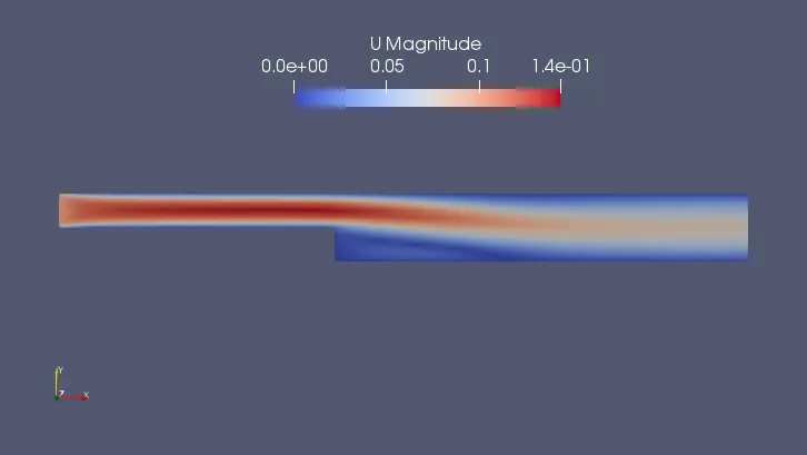
Fig. 6: Velocity contour with grading factor GF = 1 (left); and GF = 0.2 (right)
The flow through the inlet section is laminar and the velocity is high near the center and lowers towards the walls due to the no-slip condition. Once the flow crosses the step wall, the flow loses energy, and the velocity decreases as the flow progresses. There are minor vortices formed near the step wall and at the top of the wall which dissipates as the flow approaches steady-state.
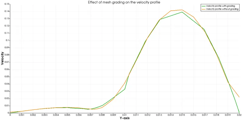
Fig. 7: Comparison of velocity profiles for GF = 1 (orange); and GF = 0.2 (green)
As we can see from Fig. 7, the velocity profiles are affected due to grading factor. The highest velocity is lower in the case of GF '0.2'.