Supervised Learning - Prediction Week 3 Challenge

1) Perform Gradient Descent in Python with any loss function

Gradient Descent is performed using Least Mean Square Error loss function on the follwing data set,

Engine Capacity in Litres	Millege
0.8	22
1	20
1.5	16
2	12
2.5	9

The aim is to find the best fit linear line (m and b) such that it has minimum Least Mean Square Error

MSE = `1/n sum_(i=0)^n(y_i - (mx_i + b))^2`

Minimum Square error can be found by calculating its partial differentiative and moving in the direction of downward slope till it attain local minima.

`del/(delm) = 2/nsum_(i=0)^n - x_i(y_i-(mx_i+b))`

`del/(delb) = 2/nsum_(i=0)^n - (y_i-(mx_i+b))`

a) Initialize m and b = 0 

b) Set Learning rate to 0.01 and Number of iteration to 1000

c) Update m and b in each iteration using,

    b = b - learning rate * `del/(delb)`

    m = m - learning rate * `del/(delm)`

d) When cost function increased when compared to previous interation we need to stop the iteration

e) Using trail and error update the learning rate and number of iteration to find the best values for the model such that we attain the minimum MSE

To evaluate the model we calculate the `R^2`,

`R^2 = 1- (sum_(i=0)^n (haty-y_i)^2)/(sum_(i=0)^n (bary-y_i)^2)`

Code: 

import numpy as np

x = np.array ([0.8,1,1.5,2,2.5]) # Engine Capcity in Litres
y = np.array ([22,20,16,12,9])   # Millege of the Vehicle in kmpl
y_mean = np.mean(y)
n = len(x)   # Number of elements
m = 0
b = 0
cost_function_old = 0
l_rate = 0.01  # Suitable Learning Rate         
for i in range (0,10000):               # Number of iterations = 10000
    y_predicted = m*x + b               # Predicting y based on the initial values of m and b
    cost_function = (1/n)*sum(((y-y_predicted)**2))  
    if (cost_function>cost_function_old and i>0): # To check whether the cost function reached minima and started to increase
        break
    cost_function_old = cost_function
    m_d = (-2/n) * sum(x*(y-y_predicted))           # Finding the partial differtial of m and b
    b_d = (-2/n) * sum((y-y_predicted))
    m = m - (l_rate * m_d)             # Updating m and b
    b = b - (l_rate * b_d)
     
    print (i,'m = ',m,'b = ',b,'cost_function = ',cost_function)

y_predicted = m*x + b                  
R_square = 1-((sum((y-y_predicted)**2))/(sum((y-y_mean)**2)))         # Formula to calculate R^2
print('R^2 = ',R_square)

Output:

 

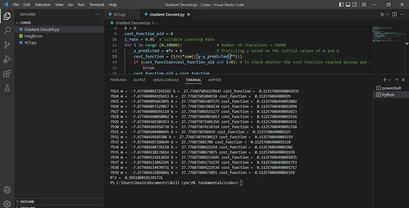
For our model we can see that cost function has reached a minimum value in 7939 iteration (learning rate = 0.01 and iteration = 10000),

`m= -7.677484115896041`

`b= 27.77687509671055`

`R^2 = 0.9951808191391731`  which means the model is a good fit (since it is close to 1)

2) Difference between L1 & L2 Gradient descent methods

L1 uses Least Absolute Deviation while L2 uses Least Mean Square Error

L1 (Least Absolute Deviation) =  `1/n sum_(i=0)^n|y_i - y_p|`

L2 (Mean Squre Error) = `1/n sum_(i=0)^n(y_i - y_p)^2`

L2 method is generally preferred because the function is continious and can be differentiable at all points but in case of L1 absolute value is not differentiable at zero

On the other hand L1 is robust to outliers but when there are outlier L2 will cause larger error since it is squared.Hence, L1 can be preferred when there are outliers in data.

3) What are the different loss functions for regression

The main loss functions are,

Mean Absolute Error =  `1/n sum_(i=0)^n|y_i - y_p|`

Mean Square Error = `1/n sum_(i=0)^n(y_i - y_p)^2`

Root Mean Square Error = `sqrt((sum_(i=0)^n(y_i - y_p)^2)/n)`

Besides these we have mean absolute percentage error, mean squared logarithmic error etc..

4) What is the importance of learning rate

Learning rate controls how much the values of m and b changes in each iteration. The learning rate decides how quickly the model gets to the local minima.

If we have high learning rate the model may skip the minima and hence resulting to incorrect behaviors.

If we have low learning rate the model will be training slowly and hence it might require lot of iteration to reach the minma.

Hence, it is important to choose optimum learning rate suitable for the model.

5) How to evaluate linear regression

Important measure to evaluate linear regression is using `R^2`

R - squared tells how much variation of dependent variable (output - Y) is explained by independent variable (Input - x) in the linear regression model

`R^2 = 1- (sum_(i=0)^n (haty-y_i)^2)/(sum_(i=0)^n (bary-y_i)^2)`

If R - squared is close to 1, then the model is a good fit

If R - squared is close to 0, then the model is a poor fit

Linear Regression models can also be evaluated based on Mean Absolute Error,Mean Square Error,Root Mean Square Error etc..

6) What is the difference between multiple and adjusted coefficient of determination

Multiple Coeffecient of determination increase whenever a new variable is added irrespective of whether it helps in improving the model i.e Multiple Coeffecient of determination increases even when a variable which is useless in determining the output is added.

Adjusted Coeffecient of determination takes into account the number of variables also. Hence, when a useful variable is added Adjusted Coeffecient of determination increases. But when a useless variable is added adjusted Coeffecient of determination decreases thus providing better insight about the model fit.