Supervised Learning - Prediction Week 3 Challenge

1.Perform Gradient Descent in Python with any loss function.

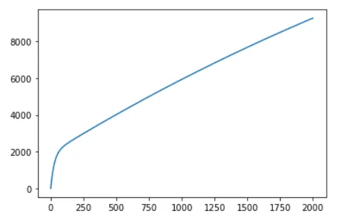
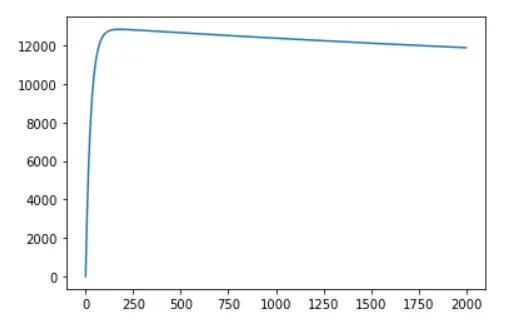
ans: i performed gradient descent in python using the loss function of sum of mean squared error. i used salary_data as the data to train the model. first i defined the function Y = lamda x*m + b. also defined plot_line to draw Y i a grapkeeping the leraning rate as 0.001 and no. of iterations of 2000,

The curve for the intercept was:

and the curve for the coefficient was:

the output line plotted over the values:

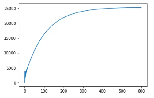
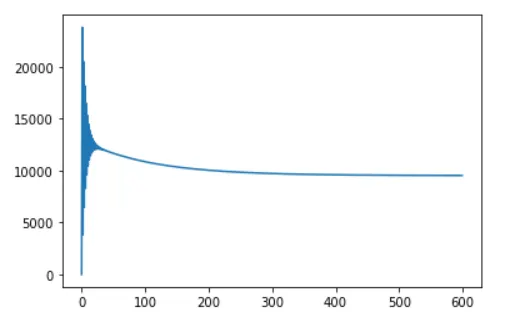
the curve for the intercept shows that the learning rate is too low. after trial and error the optimal value for learning rate(0.05) and the number of iterations(600) was found.

intercept curve:

co-efficient curve:

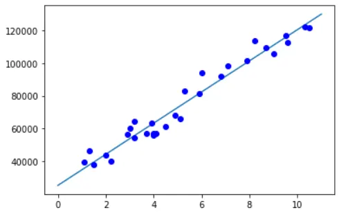
and the final output line plotted over the values is shown below.

the dataset and the program file are attached.

2. Difference between L1 & L2 Gradient descent method?

ans: the difference lies in what parameter is taken in loss fuction. L1 estimates the median of data and L2 estimates the mean of the data.L2 regularization is likely to be more accurate in all the circumstances, however, at a much higher level of computational cost.

3. What are the different loss functions for regression?

ans: Different cost functions for regression are Mean Absolute Error, Mean Squared Error, Root Mean Squared Error and Root Mean Squared Logarithmic Error.

4.What is the importance of learning rate?

ans: The learning rate decide how fast or slow the gradient arrives at the bottom of the curve. If the learning rate is too high the algorithm might overshoot the minimum and it may fail to converge and the if its too low it may take way longer to find the optimal point.

5.How to evaluate linear regression?

ans: we evaluate the regression model by using a good of fit condition. we usually use R suare or adjusted R square method.

6. What is the difference between multiple and adjusted coefficient of determination?

ans: when ever a new dependent variable is added to the model the R squared value inherently increases and is interpreted as beeter at face value while that may not be the case. to counter this adjusted R squared is used. this adds penalties to the number of new variables added and neutralises the bias caused by these variables.