Supervised Learning - Classification Week 7 Challenge

Answer 1) Pros and Cons of Support Vector Machines

Pros:

• Accuracy is good.
• More efficient because subset of training points used.
• Optimization is very good due to the convex nature of optimization function, which results in global minima instead of local minima.
• Can used for both linearly separable (hard margins) and Non-linearly separable (soft margin) data.
• SVM works relatively well when there is a clear margin of separation between classes.
• SVM is more effective in high dimensional spaces.
• SVM is effective in cases where the number of dimensions is greater than the number of samples.
• SVM is relatively memory efficient.

Cons:

• Works very on clean and small dataset.
• Support Vector Machines less efficient on noisy datasets in which classes overlapped with each other.
• It isn’t suited computationally for large dataset where number of rows exceeds a limit.
• In Natural Language Processing problem, where structured information like word embedding used for sequential data, SVM performs worst.
• Probability estimate which desired in most classification problems, SVM don’t directly provide these estimates.
• SVMs over-fit if the number of features are much more than total number of samples provided.

Answer 2) Applying SVM to analyse "Surface defects in Stainless Steel plates"

Objective: To apply Support Vector Machine (SVM) algorithm to Steel plates dataset and analysing accuracy

Steps followed:

1. Data Preparation & cleaning
2. Data Visualization
3. Finding Correlations between features
4. Analysing Outliers
5. Applying SVM
6. Conclusion

1. Data Preparation and cleaning

In this process we import libraries required

Loading dataset file

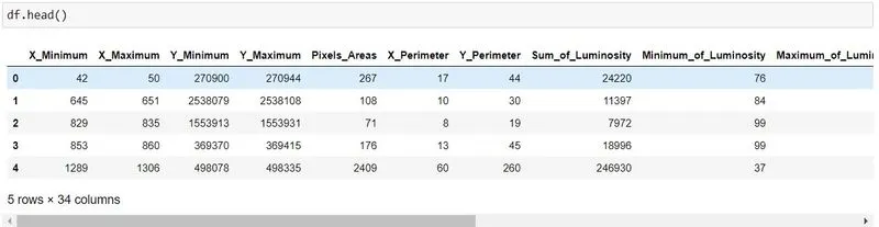
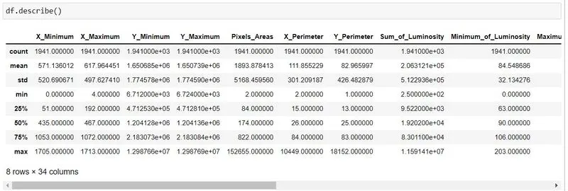
Describing the data points

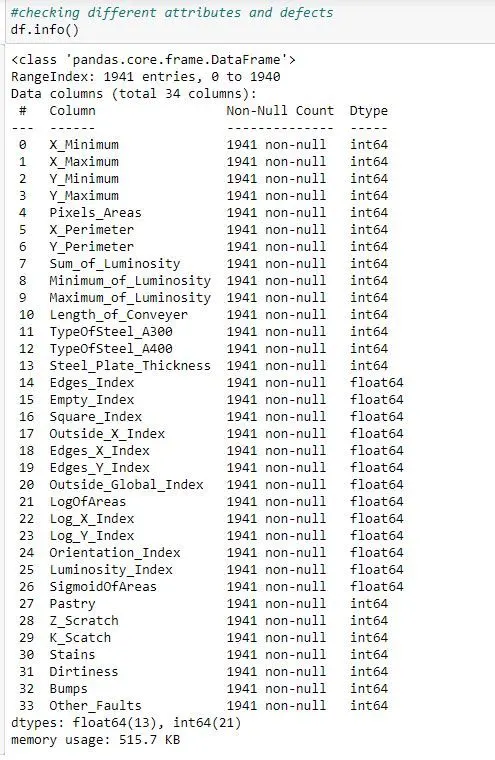
Checking different attributes and defects present in the data

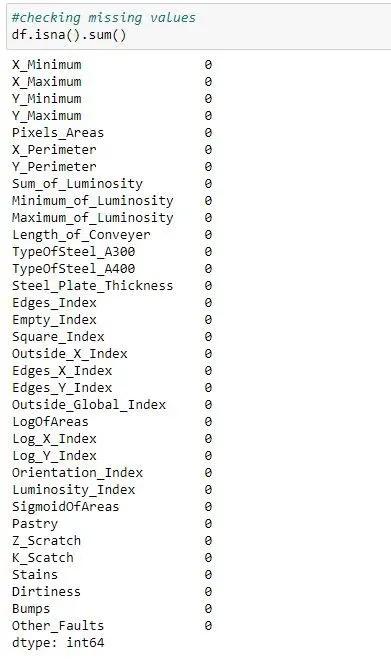
Checking null values

• There are 1941 data points and 34 features in the dataset, out of which 27 are attributes and 6 are defects
• All the values in the columns are of int and float type only
• There are no missing values present in the data

2. Data Visualisation

Plotting Piechart to visualise the data

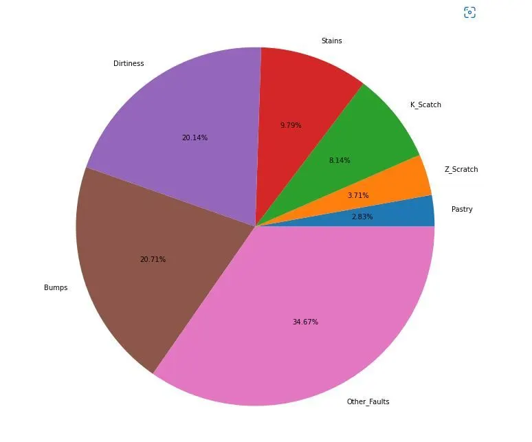
From the pie chart we can see

• Pastry Faults are minimum which amounts only 2.8%
• Other_Faults are maximum which amounts 34.67%

Now we will see distribution among attributes

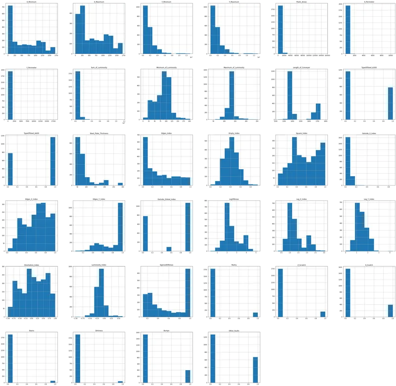
From above histogram plots we can observe that maximum number of defects occur when X dimension ranges from 0 to 250 and Y dimension ranges from 0-0.03e7

The steel plate type of A400 has more number of defects than the steel plates of type A300

Understanding relationships between features

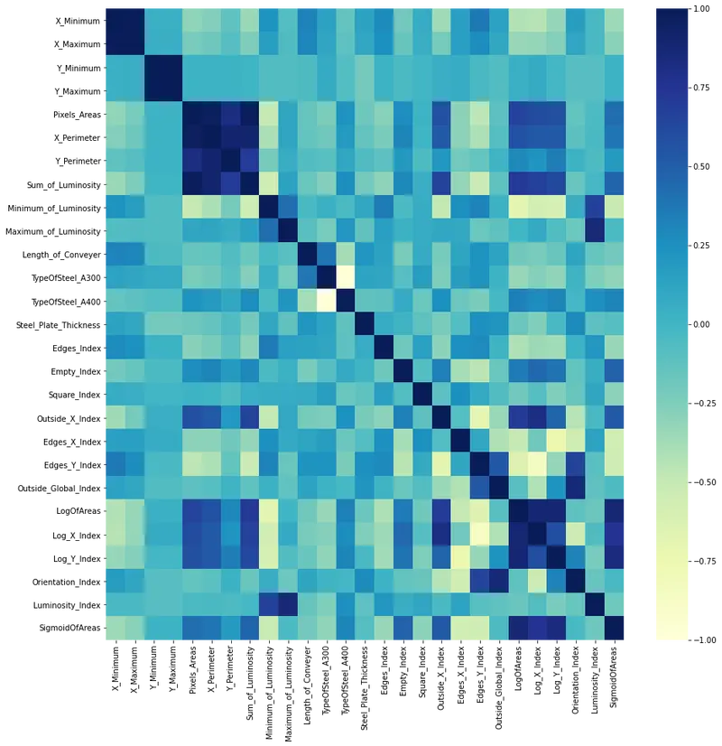
The dark colour shows strong correlation between features

we can observe the following correlations between the features

• Sum of Luminosity and Pixels Area
• Log of Areas and Sigmoid of Areas
• OrientationIndex and Outside Global Index
• Edges Y Index and Outside Global Index
• Maximum Of Luminosity and Luminosit Index

3. Finding Correlations between features

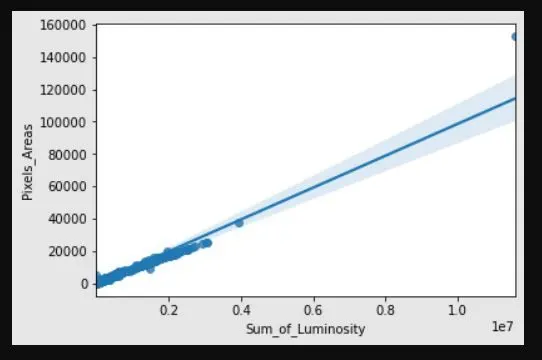
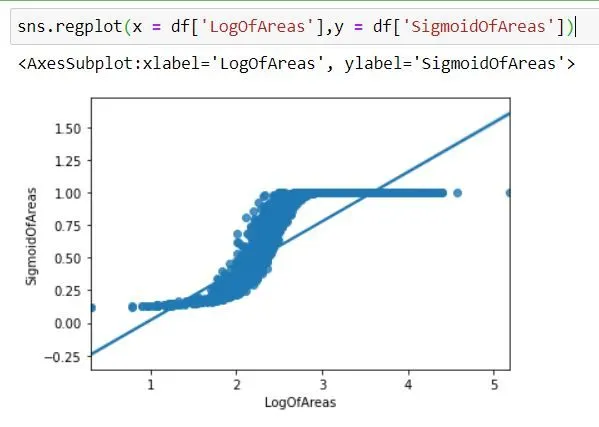
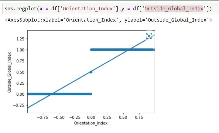
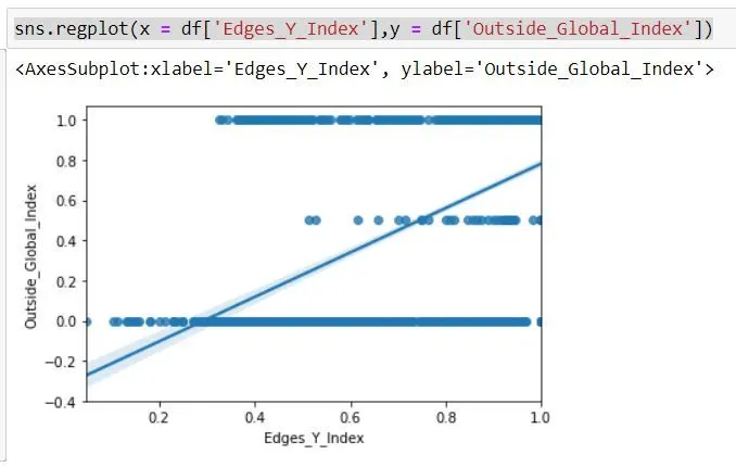
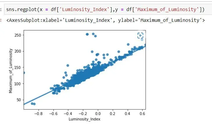
From above 5 correlations only 3 plots are shown the actual linear correlations between the features

• Sum of Luminosity and Pixels Area
• Log of Areas and Sigmoid of Areas
• Maximum Of Luminosity and Luminosit Index

4. Analysing Skewness & Outliers

We will now check each and every column which and visualise the most skewed columns

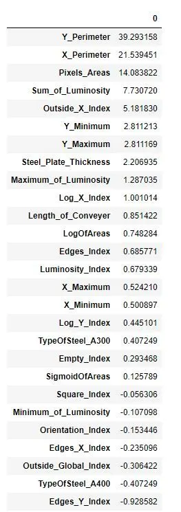
Y_perimeter is the most positively skewed column

Edges_Y_Index is the most negatively skewed column

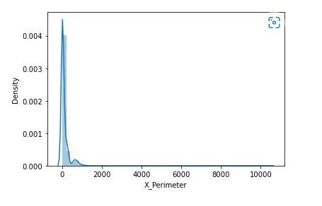
Visualising the skewness

.

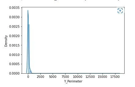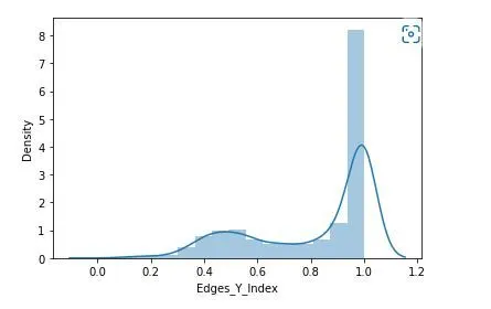
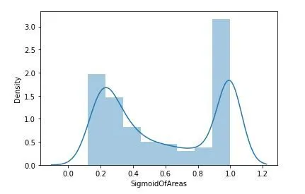
Notes:

• Y_perimeter & X_perimeter is most positive skewed features
• Edges_Y_index is the most negative skewed feature
• SigmoidOfAreas is the most normalised feature
• Most of the features are near to normal distribution

Analysing Outliers

An outlier is an observation that lies an abnormal distance from other values in a random sample from a population.

An outlier acts as a noise in the data which is not good for the machine learning algorithms to predict the model

Boxplot is the best plot for representing the outliers

We scale the data as we have large number of data points

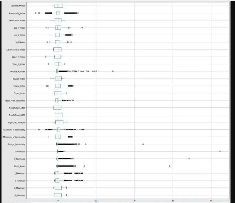
Observations: There are many outliers in this dataset which is expected as this is a fault dataset of the steelplates.

5. Applying SVM

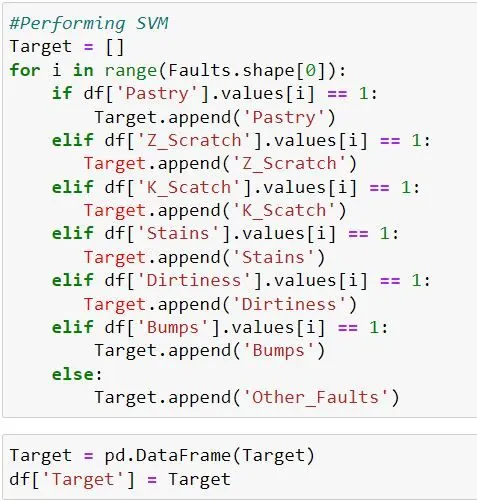
We create a new column called 'Target' in which we will merge all the faults into one column as SVM algorithm can only be performed with one target column

now we will split the data into training and testing in 70:30 % ratio

We will use Attribues_scaled dataset for further process

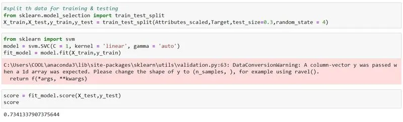
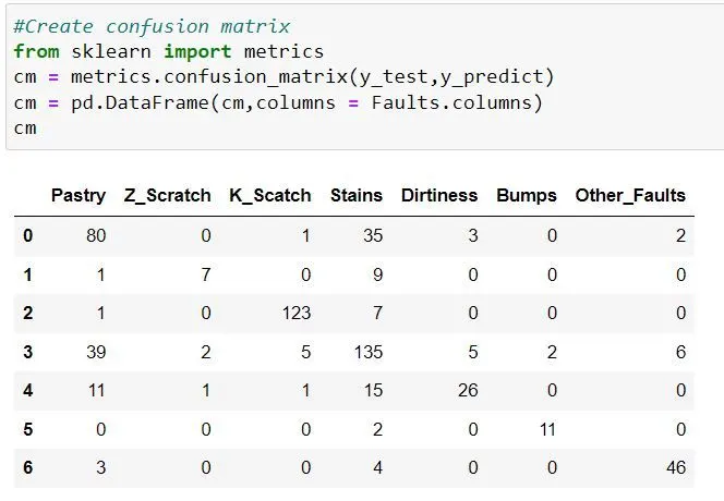
Applying SVM it gives 73.41% accuracy to our dataset

Creating confusion matrix to visualise properly

6. Conclusion

The dataset was first scaled and divided into training and testing with 70:30 ratio

The accuracy of the SVM model gives 73.41%

Confusion matrix shows most errors occur in the prediction of 'Stains' defects