Project

Study of PID controller in MATLAB.

VVikas Bhakre25 Jan 2022

Questions:

In which situations feedforward control of DC motor fails? Prepare a MATLAB script for feedforward control and test it.

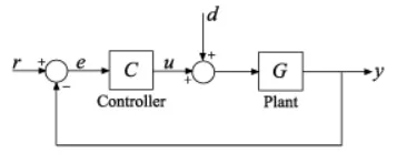
Assume a plant and a controller to prepare the same structure in Simulink as shown in the below figure. Also, use the PID Controller block in Simulink and verify system response with General Observations for PID gain:

Consider below system-

The Plant in this example is:

Plant=`frac(0.3)(s^2+0.1s)`

Use MATLAB PID tuner and prepare a table showing PID values with response time and transient behaviour coefficient.

Solution:

In which situations feedforward control of DC motor fails? Prepare a MATLAB script for feedforward control and test it.

Feedforward control of DC motor fails in following situations:

Feedforward control cannot compensate for unmeasured disturbances and any errors in the process model.
Feedforward design neglects process dynamics. How fast the controlled variable responds to the chnages in the load and manipulated variables.
A correct mathematical model should be known for exact disturbance rejection.
Feedforward controller structure will change with disturbance type and sensor used.
Recommended for slow varying process only.
Feedforward control alone cannot give desired response hence it always has to be used with a feedback controller.
The disturbance variables must be measured online. In many applications, this is not feasible.
The quality of the feedforward control depends on the accuracy of the process model.
Ideal feedforward controllers that are theoretically capable of achieving perfect control may not be physically realiable.
It's not always simple to make feedforward gain to be inverse of DC gain of plant.

Preparing the MATLAB script:

In armature controlled DC motor applies voltage Va that controls the angular velocity of the shaft.

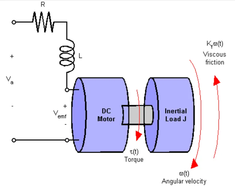
Fig01: Schematic diagram of the DC motor model of feedforward control system.

Both electrical and mechanical components are represented here, with the DC motor modeling constants as:

`T=KmIa`

`Vemf=Kbomega`

The torque T(t) and Angular velocity ω(t) are what we are intrested in:

Electrical:

`Va=IaRa+L(deli)/(delt)+Vemf`

`Va-Vemf=frac(T)(Km)(Ra+Ls)`

`T=frac(Km)(Ra+Ls)(Va-Vemf)`

Mechanical:

`T=J(delomega)/(delt)+Tload`

`T=J(delomega)/(delt)+Kfomega`

`T=omega(Js+Kf)`

`omega=frac(T)(Js+Kf)`

A simplified model of DC motor is shown above. The Torque (Td) models the load disturbances. You must minimize the speed variations induced by such disturbances.

Matlab Script:

%% DC Motor Control
% This example shows the comparison of three DC motor control techniques
% for tracking setpoint commands and reducing sensitivity to load
% disturbances:
%
% * feedforward command
% * integral feedback control
% * LQR regulation
%
% See "Getting Started:Building Models" for more details about the DC
% motor model.

%   Copyright 1986-2014 The MathWorks, Inc.

%% Problem Statement
% In armature-controlled DC motors, the applied voltage Va controls the
% angular velocity w of the shaft.
%
% <<../dcdemofigures_01.png>>
%
% This example shows two DC motor control techniques for reducing the
% sensitivity of w to load variations (changes in the torque opposed by the
% motor load).
%
% <<../dcdemofigures_02.png>>
%
% A simplified model of the DC motor is shown above. The torque Td
% models load disturbances. You must minimize the speed variations
% induced by such disturbances.
% 
% For this example, the physical constants are:

R = 2.0;                % Ohms
L = 0.5;                % Henrys
Km = 0.1;               % torque constant
Kb = 0.1;               % back emf constant
Kf = 0.2;               % Nms
J = 0.02;               % kg.m^2/s^2

Constructing a state-space model of the DC motor with two inputs (Va,Td) and one output (w):

%%
% First construct a state-space model of the DC motor with two inputs
% (Va,Td) and one output (w):

h1 = tf(Km,[L R]);            % armature
h2 = tf(1,[J Kf]);            % eqn of motion

dcm = ss(h2) * [h1 , 1];      % w = h2 * (h1*Va + Td)
dcm = feedback(dcm,Kb,1,1);   % close back emf loop

%%
% Note: Compute with the state-space form to minimize the model order.

%%
% Now plot the angular velocity response to a step change in voltage Va:
%
stepplot(dcm(1));

%%
% Right-click on the plot and select "Characteristics:Settling Time" to
% display the settling time.

Step response plot:

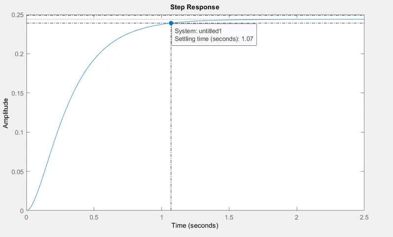
Fig02: Step response without any controller.

Observation:

The step response is following the amplitude of 0.25. The settling time is 1.07 seconds and Steady state at amplitude of 0.24.

Therefore it's clear that the step response is never gonna achieve the amplitude of 1. In order to do so the DC motor system requires a high gain control system.

Feedforward DC motor Control System:

Feedforward control is nothing but applying simple gain before the model.
Va is now presetted with Kff, so Kff is feedforward gain.
Feedforward gain is exact inverse value of the DC gain of the plant.
We can use this simple feedforward control structure to command the angular velocity ω to a given value ω_ref.

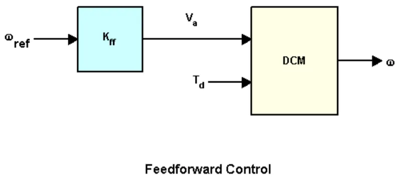
Fig03: Feedforward control system structure.

The feedforward gain Kff should be set to the reciprocal of the DC gain from Va to w.

%% Feedforward DC Motor Control Design
% You can use this simple feedforward control structure to command 
% the angular velocity w to a given value w_ref. 
%
% <<../dcdemofigures_03.png>>
%
% The feedforward gain Kff should be set to the reciprocal of the DC gain
% from Va to w.
%
Kff = 1/dcgain(dcm(1))

System is modified as we apply Kff = 4.1
System is modified by considering the values Kff and 1.
Cl_ff is another transfer function that is closed loop and feedforward where Kff is multiplied with diameter.
Adding feedforward gain to the diagonal elements of matrice 'A' is going to become Cl_ff.

To evaluate the feedforward design in the face of load disturbances, simulate the response to a step command w_ref=1 with a disturbance Td = -0.1Nm between t=5 and t=10 seconds:

%%
% To evaluate the feedforward design in the face of load disturbances,
% simulate the response to a step command w_ref=1 with a disturbance Td =
% -0.1Nm  between t=5 and t=10 seconds:
%
t = 0:0.1:15;
Td = -0.1 * (t>5 & t<10);       % load disturbance
u = [ones(size(t)) ; Td];       % w_ref=1 and Td

cl_ff = dcm * diag([Kff,1]);    % add feedforward gain
cl_ff.InputName = {'w_ref','Td'};
cl_ff.OutputName = 'w';

h = lsimplot(cl_ff,u,t);
title('Setpoint tracking and disturbance rejection')
legend('cl_ff')

% Annotate plot
line([5,5],[.2,.3]); 
line([10,10],[.2,.3]);
text(7.5,.25,{'disturbance','T_d = -0.1Nm'},...
            'vertic','middle','horiz','center','color','r');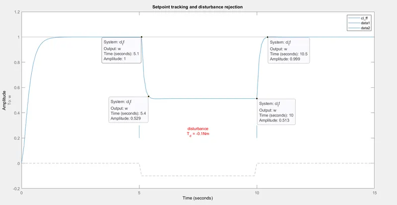

Fig04: Setpoint tracking and Disturbance Rejection plot.

Observations:

Although all the characteristics such as Rise time, Settling time and Steady State error are improved but the output plot also shows, How poor the response is to external disturbance.
Adding the disturbance by introducing torque of -0.1 N.m of load torque in the opposite direction of the DCM completely changes the step response between 5-10 seconds. The system is unable to reject the disturbance and hence is unstable in that time interval.
Due to this external disturbance the amplitude of angular velocity fails to track the set point.
Feedforward works well and increases the angular velocity from point 0.25 to 1.
Steady state also occurs within enough amount of settling time but disturbance is not rejected.
This is the limitation of feedforward control system. As soon as there appears disturbance that is unaccounted for, the system becomes unstable as there is no sensor to detect the error and adjust the system accordingly using feedback control. Therefore it is not recommended.

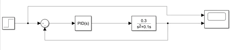
Fig05: Simulink model for PID tuning.

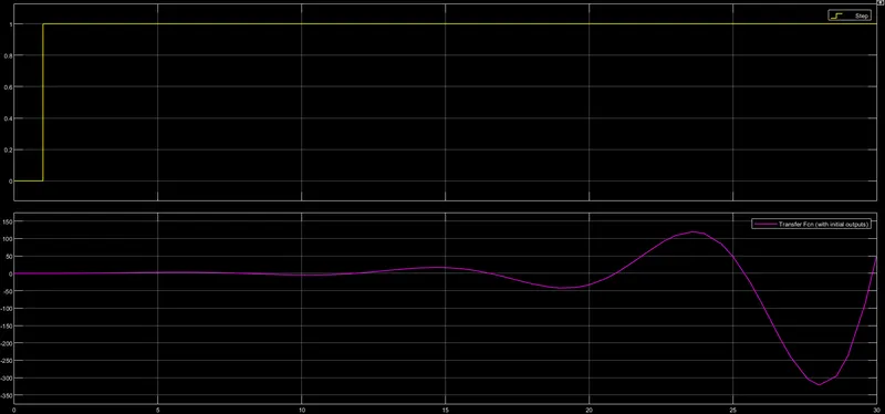
Fig06: Default (untuned) results for simulink model of PID tuning.

From the results it is clear that the step response of this transfer function is unstable, as it continues to rise with time.
Default values of Praportional (Kp), Integral (Ki) and Derivational (Kd) constants of the PID controller are:
Praportional constant (Kp) = 1
Integral constant (Ki) = 1
Derivational constant (Kd) = 0

Tuning PID controller to stabalize the system:

In order to stabalize the system we must change the values of Praportional (Kp), Integral (Ki) and Derivational (Kd) constants of the PID controller.

Test: I]

Praportional constant (Kp) = 10
Integral constant (Ki) = 10
Derivational constant (Kd) = 05

Here we are introducing the value of Derivational constant (Kd) = 05 therefore the phase of the output of the step response changes.

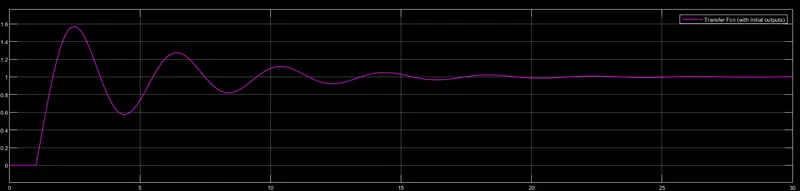
Fig07: Tuned PID results for simulink model of PID tuningfor Test I.

Test: II]

Praportional constant (Kp) = 20
Integral constant (Ki) = 20
Derivational constant (Kd) = 05

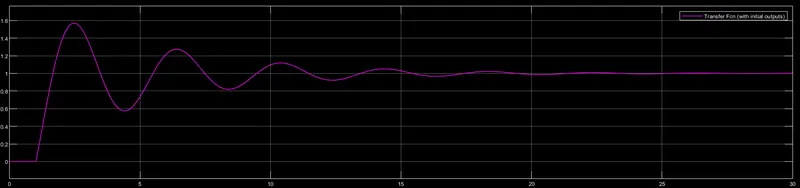
Fig08: Tuned PID results for simulink model of PID tuningfor Test II.

Test II] results:

Rise time is reduced.
Settling time is reduced.
Overshoot is increased.
Steady state error is reduced.

Test: III]

Praportional constant (Kp) = 50
Integral constant (Ki) = 50
Derivational constant (Kd) = 05

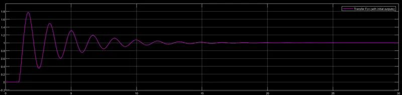
Fig09: Tuned PID results for simulink model of PID tuningfor Test III.

Test III] results:

Rise time is reduced.
Settling time is reduced.
Overshoot is increased.
Steady state error is reduced.

Test: IV]

Praportional constant (Kp) = 100
Integral constant (Ki) = 100
Derivational constant (Kd) = 10

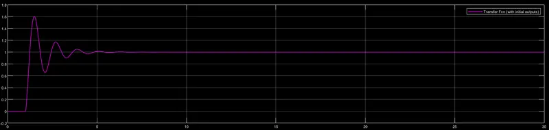
Fig10: Tuned PID results for simulink model of PID tuningfor Test IV.

Test IV] results:

Minimal change inRise time.
Settling time is reduced.
Overshoot is increased.
Steady state error is reduced.

Observations of PID gain:

Gain	Rise Time	Overshoot	Settling Time	Steady State Error
Kp	Decrease	Increase	Small change	Decrease
Ki	Decrease	Increase	Increase	Eliminate
Kd	Small change	Decrease	Decrease	Small change

Consider below system-

The Plant in this example is:

Plant=`frac(0.3)(s^2+0.1s)`

Use MATLAB PID tuner and prepare a table showing PID values with response time and transient behaviour coefficient.

Matlab script:

clear all
close all
clc

% Defining the transfer function G.

num = [0.3];
den = [1 0.1 0];
G_tf = tf(num,den)

pidTuner(G_tf)

Case I] Default:

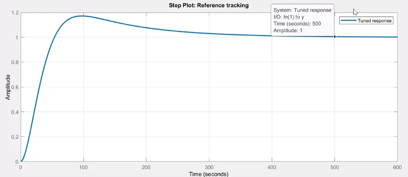
Fig11: Default untuned PID results for simulink model of Plant.

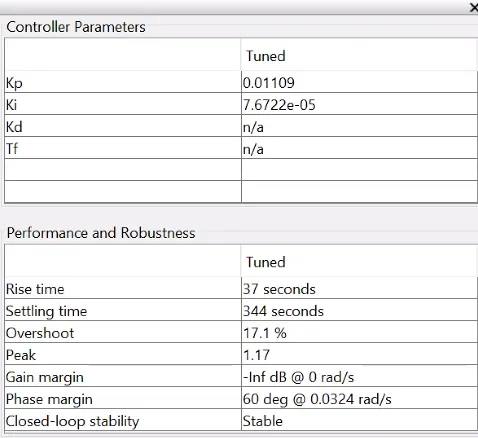
Fig12: Default vakues of Kp ,Ki and Kd of Plant transfer function.

Case II]

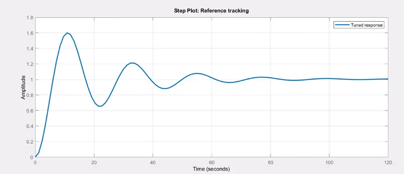
Fig13: Default untuned PID results for simulink model of Plant.

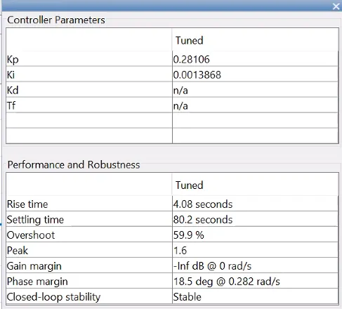
Fig14: Tuned values of Kp ,Ki and Kd of Plant transfer function.

Values of Kp and Ki are increased.

Which results in:

Decrease in rise time.

Decrease in settling time.

Increase in overshoot.

Case III]

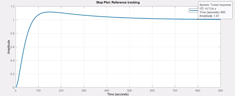
Fig15: Default untuned PID results for simulink model of Plant.

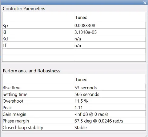
Fig16: Tuned values of Kp ,Ki and Kd of Plant transfer function.

Values of Kp and Ki are decreased.

Which results in:

Increase in rise time.

Increase in settling time.

Decrease in overshoot.

Conclusion:

Feedforward control system is easy to implement but has lots of limitations.
Changing the values of Kp, Ki and Kd is a convinient method of making the system stable

Study of PID controller in MATLAB.

Ship work like this
in your own course.

Talk to a career counsellor

Ship work like thisin your own course.

Talk to a career counsellor

Ship work like this
in your own course.