Developing Code using MATLAB for studying numerical dissipation and dispersion errors of hyperbolic (linear convection) equation.
Aim- Study of numerical dissipanion and dispersion of hyderbolic (linear convection) equation.
Theory-
From our previous project It was well understood that all numerical scheme has up to some degree of accuracy considering truncation error and round off errors. In this we will focus on different aspect of difference equation apart from truncation error and round off errors.
The model equation for this challenging will be taken as 1-D linear convection equation with following specification i.e
`(delu)/(delt)+a((delu)/(delx)) = 0`------------------(1)
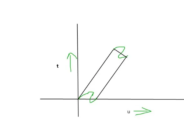
`u = f(x-at) " a>0"`
`u = f(x+at)` a<0
Refering to Von- Neuman stability analysis when local transport property moves right side from reference axis(i.e wave speed a > 0 ) first order reward difference in space gives stable solution having said that we can discretize our model equation explicitely 1st order backward in space. so our difference equation will be-----
`(u_i^(t+Deltat)-u_i^t)/(Deltat)+a(u_i^t-u_(i-1)^t)/(Deltax) = 0` ---------------------(2) `
From our previous observation we can say the above difference equation is 1st order accurate in time and space [`O(Deltat,Deltax)`].Rearranging the equation 2 we can write --------
`(u_i^(t+Deltat))/(Deltat) = u_i^t-k(u_i^t-u_(i-1)^t)`
Where`k = a((Deltat)/(Deltax))`which is called as Courant–Friedrichs–Lewy number. Solving The above equation explicitely in MATLAB we can get the following Plots.
Matlab Code
clear all
close all
clc
% calculation of linear convection
l =1;
n = 20;
c = 1;
dt = .01;
% calculation
x = linspace(0,l,n);
dx = x(2)-x(1);
nt = .4/dt;
x_start = 0.1;
x_end = 0.3;

cfl = (c*dt/dx);
% time loop

for p = 1:length(x)
    if x(p) >= .1 && x(p)<=.3
         u(p) = 2;
    else
        u(p)=1;
    end


   end
u_initial = u;
u_old=u;
for k = 1:nt
    %space loop
    for i = 2:n
        u(i) = u_old(i)-cfl*(u_old(i)-u_old(i-1));
    end
    % update old velocities
    u_old = u;
    % plotting the velocities
    grid on
    plot(x,u_initial,'r')
    hold on
    plot(x,u,'b')
    axis([0 1 0 3])
    pause(.3)
end
Plots
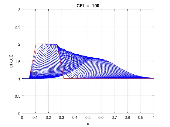
1. when grid (n) = 20)
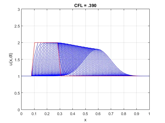
2. when grid (n) = 40
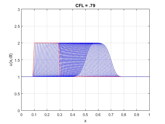
3. when grid (n) = 80
4. when grid (n) = 160
Case-2
As a function of time step (dt)
No of grid = 80
dt = [1e-4, 1e-3, 1e-2, 1e-1]
Matlab code
Main code
clear all
close all
clc
% calculation of linear convection
l =1;
n = 80;
c = 1;
t = 0.4;
dt = [1e-4 1e-3 1e-2 1e-1];
% calculation
x = linspace(0,l,n);
dx = x(2)-x(1);
x_start = 0.1;
x_end = 0.3;
n_start = round((x_start/dx)+1);
n_stop = round((x_end/dx)+1);
u =1*ones(1,n);
u(n_start:n_stop)= 2;
u_old = u;
u_initial = u;

cfl1 = (c*dt(1)/dx);
cfl2 = (c*dt(2)/dx);
cfl3 = (c*dt(3)/dx);
cfl4 = (c*dt(4)/dx);

u1 = tmestp(t,dt(1),x,u_old,c);
u2 = tmestp(t,dt(2),x,u_old,c);
u3 = tmestp(t,dt(3),x,u_old,c);
u4 = tmestp(t,dt(4),x,u_old,c);
% plotting the velocities

subplot(5,1,1)
grid on
plot(x,u_initial,'r')
xlabel('x')
ylabel('U(x,t)')
legend('initial function')
hold on
subplot(5,1,2)
plot(x,u1,'b')
pause(.3)
xlabel('x')
ylabel('U(x,t)')
title('CFL = .0079')
subplot(5,1,3)
plot(x,u2,'b')
pause(.3)
xlabel('x')
ylabel('U(x,t)')
title('CFL = .079')
subplot(5,1,4)
plot(x,u3,'b')
pause(.3)
xlabel('X')
ylabel('U(x,t)')
title('CFL = .79')
subplot(5,1,5)
plot(x,u4,'b')

xlabel('x')
ylabel('U(x,t)')
title('CFL = 7.9')
pause(.3)
axis([0 1 0 3])
hold on
Function
function u = tmestp(t,dt,x,u_old,c)

    n = length(x);
    dx = x(2) - x(1);
    nt = t/dt;
    cfl =(c*dt/dx);
    for k = 1:nt
        %space loop
        for i = 2:n
            u(i) = u_old(i)-cfl*(u_old(i)-u_old(i-1));
        end

        u(1) = 1;

        % update old velocities
        u_old = u ;

    end

end
Plot 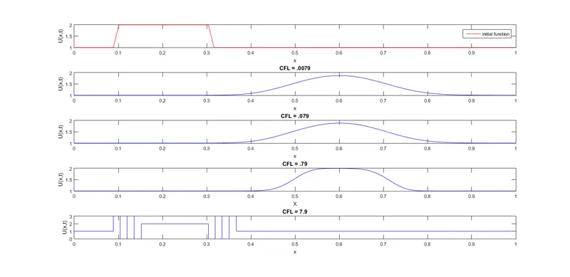
Observation & Conclusion
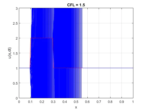
1. When the grid number is 20, and we can see the peak is dying very fast in due course of propagation which should not be in reality meanwhile if we look the remaining three cases at n=40, peak is slowly dying, followed by n=80 but it is getting unstable when grid spacing tends to very very small value here we can see that behaviour at n=160.
From case-2 When the CFLnumber is .0079, we can see the peak is dying very fast in due course of propagation which should not be in reality meanwhile if we look the 3rd sub plot at CFL = .79, peak is slowly dying, but it is getting unstable when CFL = 7.9
2. To answer what makes its peak to die down and blown upon solution in some cases let’s see modified wave equation.
 --------------------------------------(4)
3. Equation (4) gives us some information on the behaviour to be expected from the numerical solution of the difference equation . Examining equation (4) closely we can make analogy of Navier stakes equation with above modified wave equation . The term multiplied `(del^2u)/(delx^2)`in Navior-Stokes equation is viscosity, that represents dissipasive aspect of the follow.
4. similarly the term attached to`(del^2u)/(delx^2)` in our modified wave equation behaves like dissipative term in Navier-Stokes equation. However this term is a consequence of the numerical discretizasion embaided in the difference equation and therefore purely numerical origin. with no physicalsignificance. So the appearance of this term with the frame work of numerical solution is called numerical dissipation.
5. the coefficient term such as `a((Deltax)/2)(1-nu)` act much like physical viscosity and therefore is called artificial viscosity. The presence of artificial viscosity is by default embedded in our difference equation that is why peak get dies in due cource of propagation.
At
Case-1
dt = 1e-2
n--->20 CFL = .190
n--->40 CFL = .39
n--->80 CFL = .79
n--->160 CFL = 1.59
Case-2
No of grid = 80
dt = [1e-4, 1e-3, 1e-2, 1e-1]
CFL = .190 --------> Artificial viscosity- 1-.0079 = .9921
CFL = .190 --------> Artificial viscosity- 1-.079 = .921
CFL = .190 --------> Artificial viscosity- 1-.79 = .21
CFL = .190 --------> Artificial viscosity- 1-7.9 = -6.9
(i)From the above trend we can observe as ‘n’ increases CFL value increases resulting decrease in artificial viscosity. that is the reason why peak is reducing slowly while increasing grid number.
(ii) From the above trend we can observe as CFL value increases resulting decrease in artificial viscosity. that is the reason why peak is reducing slowly while increasing time step.
But at certain value i.e at n=160, wiggles starts to from at the front and behind the wave. this behaviour is called numerical disperision from modified wave equation. Numerical dispersion is the direct result of the odd order derivatives (`(del^3u)/(delx^3)` etc.). This gives a very good observation that CFL number less than 1 provides a stable solution in explicit method for Hyperbolic equation. which can be seen in Von-Neuman stability analysis.
6 . So from the above analysis we can conclude when the leading term of the truncation error is an even order derivative , the numerical solution wil display dissipstive behaviour and when the leading term is an odd order derivative , the solution will display dispersive behaviour.
Both the behaviour combiningly together called as Numerical diffusion.