1D linear convection for varying time-steps using MATLAB

OBJECTIVE:

1. To write a function that accepts the time step as an argument and solve the 1D Convection Equation. Also, to study the effect of time step size on the numerical solution.
2. To study the CFL criteria that govern the linear convection equation and see if this criterion applies to an implicit solution.
3. To explain how the change in time step size affects numerical diffusion, instability, the courant number, and accuracy.
4. To plot the simulation time as a function of the time step.

THEORY:

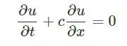
From the Navier Stokes equation, only the accumulation and convection terms for the x-component of the velocity are taken. The equation is -

• 1D, as it has got derivative w.r.t one spatial axis.
• Linear, as the coefficient of the first derivative of the velocity, is constant.
• Convective, as c.(δu/δx), is similar to the convective term Navier-Stokes equation for momentum.

The equation represents the propagation of a wave without change of shape, the speed of the wave is 'c', and with the initial condition given as-

u(x,0) = u₀

The exact solution is -

u(x,t) = u₀(x - c.t)

This means that on an axis with the positive direction to the right, the wave will move from left to right with the speed 'c'.

The equation is solved using the 'time-marching procedure', where we start with an initial condition 't=1'. We take this value and do a time marching and compute the velocity profile at 't=2', and we do this till 't=n'.

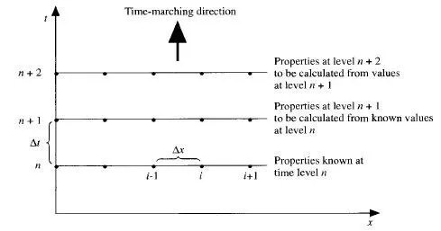
To discretize this equation in space and time we use the Forward Difference Scheme for time derivative and Backward Difference Scheme for space derivative. For time steps we use the superscript 'n' and for the space steps (grid cells), we use the subscript 'i'. The discretized form of the equation, therefore, is -

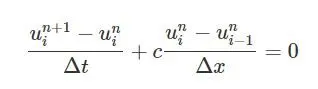
where 'n+1' and 'n' are two consecutive steps in time and 'i' and 'i-1' are two neighboring points of the discretized x coordinate (grid points). The only unknown in the equation is, therefore 'u_iⁿ⁺¹'. We solve for this unknown to get an equation that allows us to advance in time, which is as follows -

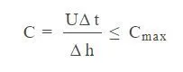
Courant Number: The Courant Number broadly indicates how much information travels 'u' across a computational grid cell 'Δh' in a unit of time 'Δt'. It is a non-dimensional number after the mathematician Richard Courant and is linked to the Courant-Friedrichs-Lewy (CFL) stability condition of numerical schemes. The Courant number formula is given as -

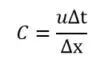
If the Courant number is greater than one, it means that the information propagates through more than one grid cell at each time step, making the solution inaccurate and potentially leading to non-physical results or divergence of the solution in certain integration schemes.

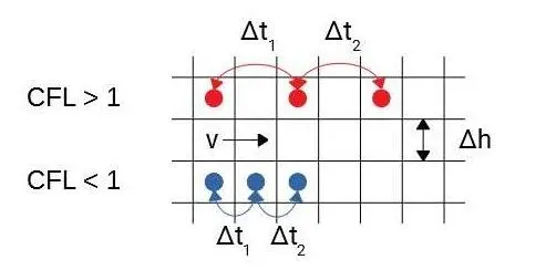
From a numerical viewpoint, the time integration schemes can be broadly divided into three groups: explicit, implicit, and semi-implicit. Roughly speaking, in explicit schemes, the solution at the time step 'n+1' is calculated using the known values of the solution at the time 'n'. Conversely, in an implicit scheme, the solution at the time 'n+1' is calculated using unknown values of the solution at the time 'n+1', hence requiring the solution of an ODE. Lastly, semi-implicit schemes use both the solution at the time 'n' and 'n+1'.

In order to converge explicit and semi-implicit schemes, the time step size needs to be carefully selected, otherwise, the simulation might lead to non-physical results or diverge altogether. The stability requirements of time-integration schemes can be defined using the Courant-Friedrichs-Lewy (CFL) condition, which takes its name after Richard Courant, Kurt Friedrichs, and Hans Lewy.

The condition is expressed in terms of the Courant number as -

INPUT DATA: The initial velocity profile is a step function. It is equal to 2m/s between x= 0.1 and 0.3 and 1m/s everywhere else.

• Domain Length, L = 1;
• Time step , dt = 1e-4, 1e-3, 1e-2, and 1e-1
• No.of grid points, n = 80;
• Convection coefficient, c = 1;
• Simulation run time, t = 0.4;

CODE:

1. Function

function [x,u] = Time_steps(dt)

% Inputs for the linear convection problem

L = 1; % Domain Length
n = 80; % No.of grid points
c = 1; % convection coefficient
t = 0.4; % Simulation run time
nt = t/dt;

    for i = 1:length(dt)
        x = linspace(0,L,n);
        dx= L/(n-1);
        u = ones(1,n);

        for m = 1:length(x)
            if x(m) >= 0.1 && x(m) <= 0.3
                u(m) = 2;
            end
        end
        
        uold = u;
        
        for k = 1:nt
            for j = 2:n(i)        
                u(j) = uold(j)-(((c*dt)/dx(i))*(uold(j)-uold(j-1)));
            end
        uold = u; % updating velocity for each time step
        end
    end
end

2. Main Code

clear all
close all
clc


% timeit, Measure time required to run function
[x1,u1]= Time_steps(1e-1);
f1 =@() Time_steps(1e-1);
t1=timeit(f1); 

[x2,u2]= Time_steps(1e-2);
f2 =@() Time_steps(1e-2);
t2=timeit(f2);

[x3,u3]= Time_steps(1e-3);
f3 =@() Time_steps(1e-3);
t3=timeit(f3);

[x4,u4]= Time_steps(1e-4);
f4 =@() Time_steps(1e-4);
t4=timeit(f4);

figure(1)
plot(x1,u1,'linewidth',1.5)
hold on
plot(x2,u2,'r','linewidth',1.5)
hold on
plot(x3,u3,'g','linewidth',1.5)
hold on
plot(x4,u4,'k','linewidth',1.5)
xlabel('Length of Domain, L');
ylabel('Velocity, m/s');
grid on
axis([0 1 0 2.5])
legend('1e-1','1e-2','1e-3','1e-4')
title('Effect of time step dt on the Velocity profiles');

figure(2)
simulation_time = [t1, t2, t3, t4];
bar(simulation_time); 
xticklabels({'1e-1','1e-2','1e-3','1e-4'});
xlabel('Time step');
ylabel('Simulation Time');
title('Time difference between time steps');
grid on

L = 1; 
n = 80; 
c = 1;
t = 0.4; 
dt = [1e-1, 1e-2, 1e-3, 1e-4];

for i = 1:length(dt)
    dx= L/(n-1);
    courant_number(i) = c*dt(i)/dx;
end

figure(3)
plot(dt,courant_number,'k','marker','o')
grid on
axis([-0.01 0.11 -0.5 8.5])
xlabel('time step size, dt')
ylabel('Courant Number, C')
title('Effect of time step size on the Courant Number')

RESULTS:

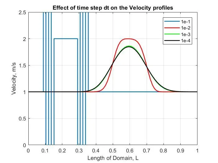
Figure 1

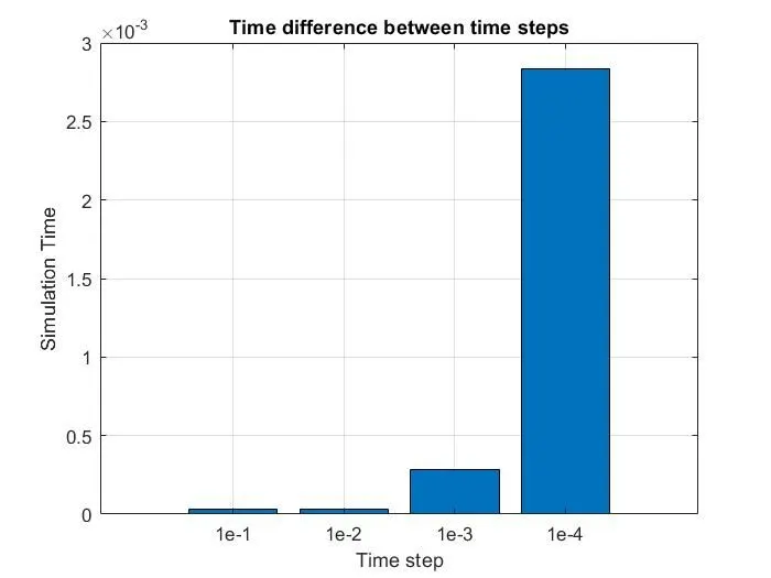
Figure 2

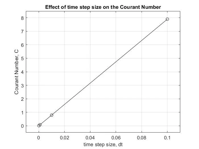
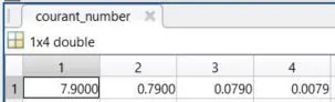
Figure 3

CONCLUSION:

In Figure 1, we observe the initial and final velocity profiles of the numerical solution for all values of dt. We see that for the time step '1e-1', the solution is unstable and blows up. This is because the Courant Number for this is 7.9 (Figure 3), which is greater than 1. For time step '1e-2', the solution is more accurate and produces a square wave, this is due to the Courant Number being 0.79 which is close to 1. For time steps '1e-3' and '1e-4', the Courant Number values are 0.079 and 0.0079 respectively, and creates artificial diffusion, causing the velocity profiles to lose their sharpness, gradient, and peak velocity.

In Figure 2, the simulation time is plotted as a function of the time step. It is seen that as the time step decreases, the simulation time increases as more computations are done to reach a particular value with smaller increments.

Also, implicit linear convection is unconditionally stable, and also lacks a CFL condition. This happens because implicit schemes use the entire domain to calculate each timestep. However, implicitly calculating (i.e., solving an implicit linear system) each timestep can be very time-consuming and costly. In addition, time accuracy decreases as the timestep increases. Therefore, it is logical is to use an explicit scheme with a lower timestep.