Structural dynamics
1. Differentiate Static analysis and Dynamic analysis with proper representing pictures
Answer:-
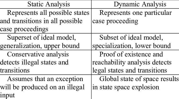
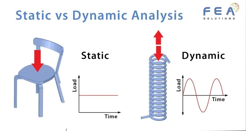
Difference between dynamic code analysis and static code analysis
Static analysis is the testing and evaluation of an application by examining the code without executing the application whereas Dynamic analysis is the testing and evaluation of an application during runtime.
Many software defects that cause memory and threading errors can be detected both dynamically and statically. The two approaches are complementary because no single approach can find every error.
The primary advantage of dynamic analysis: It reveals subtle defects or vulnerabilities whose cause is too complex to be discovered by static analysis. Dynamic analysis can play a role in security assurance, but its primary goal is finding and debugging errors.
Level of in-depth review
The key difference between a static and dynamic code analyser is the how in-depth the code review
process is. By default, static code analysis combs through every single line of source code to find flaws and errors. For dynamic analysis, the lines of code that get reviewed depend upon which lines of source code are activated during the testing process. Unless a line of code is interacted with, the dynamic analysis tool will ignore it and continue checking active codes for flaws. As a result, dynamic analysis is a lot quicker since it is able to review code on the fly and generates real-time data. However, static code analysis provides peace of mind that each and every line of source code has been thoroughly inspected. It may take longer, but static code analysis runs in the background and is crucial for creating a flawless web application.
Catching errors early and making recommendations
The primary advantage of static analysis: It examines all possible execution paths and variable values, not just those invoked during execution. Thus static analysis can reveal errors that may not manifest themselves until weeks, months or years after release. This aspect of static analysis is especially valuable in security assurance, because security attacks often exercise an application in unforeseen and untested ways.
As mentioned before, dynamic analysis reviews codes during the testing process and generates real-time results. While it is great for fine-tuning the user experience, it has one major drawback: any errors highlighted by dynamic code analysis tools requires developers to go all the way back to the source code, make changes to the code itself and then make changes to everything that has been modified as a result of changing the source code. This is a very time consuming and expensive process; one that companies and developers like to avoid at all costs. Static code analysis tools highlight any errors immediately and allow developers to makes changes before proceeding any further. Moreover, static code analysis tools are more feature-packed than their dynamic counterparts. One important feature is the number of errors it can detect and the recommendations it can make to fix that error. If configured, static code analysers can automatically make the required changes and let developers know what changes have been made.
Cost of code analysis tools
Just like any other business, software application companies have to find a fine balance between application costs and profit margins. With respect to price, static code analysis tools are always cheaper than dynamic analysers. Moreover, having a dynamic code analyser requires a company to hire professionals trained in the use of dynamic analysis tools. A static code analysis tool can be used by any web developer with ease, thus guaranteeing that it won’t turn out to be a long-term expenditure.
Static code analysers are absolutely essential for application developers, whereas dynamic code analysers can only be used in conjunction with static analysis tools.
2. Explain the following with relevant force-displacement graph
- Elastic behavior
- Inelastic behavior
- Plastic behavior
- Non-linear Inelastic behavior
Answer:-
1.Elastic behavior
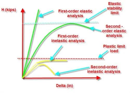
Solids are made up of atoms based on their atomic elasticity (or molecules). They are surrounded by other atoms of the same kind, which are maintained in equilibrium by interatomic forces. When an external force is applied, these particles are displaced, causing the solid to deform. When the deforming force is removed, interatomic interactions cause the atoms to return to their original state of equilibrium. Elasticity is an idealization since no substance is perfectly elastic. For example, if you use a hair tie to maintain yourself, you may have seen that its size deforms over time. It may snap after a certain point. This is because the hair tie loses its elastic nature over time.
The solids are accustomed to maintaining a physical shape by the virtue of which each molecule contained in it finds itself in a position of stable equilibrium, that is, there are balanced forces acting on the body from every pair of opposite directions. A rigid body is a solid object in which deformation is negligible, assumed to be zero for all practical purposes. These bodies when subjected to an external force restore their original shape after the removal of this force. The body resists the changes, until a limiting external force limit, called the elastic limit.
Any rigid object in the universe undergoes changes in its physical orientation and structure upon external force application. A rigid body either changes its length, volume or shape when an outward force is applied to it. The body retains its original shape and size upon removal of external acting forces. Therefore, elasticity is such a property of a body by the virtue of which anybody tends to regain its original shape (or) size when external forces are removed. It exhibits an opposition to change. Example: a rubber band.
Elastic behavior of solids
In the cases, where any solid body is subjected to an external force, the body is deformed and the atoms or molecules forming them are displaced from their original positions, thus being disturbed from the state of equilibrium.
The displacement causes the modification of fixed points, thus, causing a change in the interatomic as well as intra-molecular distances. Therefore, deformation can be termed as the change in the structure of any object due to the influence of a force acting upon it. The force that causes the shift in the displacement of these particles is known as the deforming force.
Since we know that every force has an equal and opposite force acting. The deforming force is opposed by the restoring force, acting in the opposite direction. This force pushes the body to regain its original position upon removal of the deforming force.
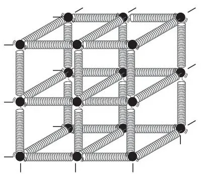
The spring ball system contains balls denoting atoms and springs representing the forces acting between them.
2.Inelastic behavior
Classical metal plasticity
-
The yield and inelastic flow of a metal at relatively low temperatures, where loading is relatively monotonic and creep effects are not important, can typically be described with the classical metal plasticity models.. In Abaqus these models use standard Mises or Hill yield surfaces with associated plastic flow. Perfect plasticity and isotropic hardening definitions are both available in the classical metal plasticity models. Common applications include crash analyses, metal forming, and general collapse studies; the models are simple and adequate for such cases.
- Models for metals subjected to cyclic loading
-
A linear kinematic hardening model or a nonlinear isotropic/kinematic hardening model can be used in Abaqus to simulate the behavior of materials that are subjected to cyclic loading. The evolution law in these models consists of a kinematic hardening component (which describes the translation of the yield surface in stress space) and, for the nonlinear isotropic/kinematic hardening model, of an isotropic component (which describes the change of the elastic range). The Bauschinger effect and plastic shakedown can be modeled with both models, but the nonlinear isotropic/kinematic hardening model provides more accurate predictions. Ratchetting and relaxation of the mean stress are accounted for only by the nonlinear isotropic/kinematic model. In addition to these two models, the ORNL model in Abaqus/Standard can be used when simple life estimation is desired for the design of stainless steels subjected to low-cycle fatigue and creep fatigue (see below).
- Rate-dependent yield
-
As strain rates increase, many materials show an increase in their yield strength. Rate dependence .can be defined in Abaqus for a number of plasticity models. Rate dependence can be used in both static and dynamic procedures. Applicable models include classical metal plasticity, extended Drucker-Prager plasticity, and crushable foam plasticity.
- Creep and swelling
-
Abaqus/Standard provides a material model for classical metal creep behavior and time-dependent volumetric swelling behavior. This model is intended for relatively slow (quasi-static) inelastic deformation of a model such as the high-temperature creeping flow of a metal or a piece of glass. The creep strain rate is assumed to be purely deviatoric, meaning that there is no volume change associated with this part of the inelastic straining. Creep can be used with the classical metal plasticity model, with the ORNL model, and to define rate-dependent gasket behavior. Swelling can be used with the classical metal plasticity model. (Usage with the Drucker-Prager models is explained below.)
- Annealing or melting
-
Abaqus provides a modeling capability for situations in which a loss of memory related to hardening occurs above a certain user-defined temperature, known as the annealing temperature.It is intended for use with metals subjected to high-temperature deformation processes, in which the material may undergo melting and possibly resolidification or some other form of annealing. In Abaqus annealing or melting can be modeled with classical metal plasticity (Mises and Hill); in Abaqus/Explicit annealing or melting can also be modeled with Johnson-Cook plasticity. The annealing temperature is assumed to be a material property. See for information on an alternative method for simulating annealing in Abaqus/Explicit.
- Anisotropic yield and creep
-
Abaqus provides an anisotropic yield model which is available for use with materials modeled with classical metal plasticity kinematic hardening and/or creep that exhibit different yield stresses in different directions. The Abaqus/Standard model includes creep; creep behavior is not available in Abaqus/Explicit. The model allows for the specification of different stress ratios for each stress component to define the initial anisotropy. The model is not adequate for cases in which the anisotropy changes significantly as the material deforms as a result of loading.
- Johnson-Cook plasticity
-
The Johnson-Cook plasticity model in Abaqus/Explicit is particularly suited to model high-strain-rate deformation of metals. This model is a particular type of Mises plasticity that includes analytical forms of the hardening law and rate dependence. It is generally used in adiabatic transient dynamic analysis.
- Dynamic failure models
-
Two types of dynamic failure models are offered in Abaqus/Explicit for the Mises and Johnson-Cook plasticity models. One is the shear failure model, where the failure criterion is based on the accumulated equivalent plastic strain. Another is the tensile failure model, which uses the hydrostatic pressure stress as a failure measure to model dynamic spall or a pressure cutoff. Both models offer a number of failure choices including element removal and are applicable mainly in truly dynamic situations. In contrast, the progressive failure and damage models are suitable for both quasi-static and dynamic situations and have other significant advantages.
- Porous metal plasticity
-
The porous metal plasticity model is used to model materials that exhibit damage in the form of void initiation and growth, and it can also be used for some powder metal process simulations at high relative densities (relative density is defined as the ratio of the volume of solid material to the total volume of the material). The model is based on Gurson's porous metal plasticity theory with void nucleation and is intended for use with materials that have a relative density that is greater than 0.9. The model is adequate for relatively monotonic loading.
- Cast iron plasticity
-
The cast iron plasticity model is used to model gray cast iron, which exhibits markedly different inelastic behavior in tension and compression. The microstructure of gray cast iron consists of a distribution of graphite flakes in a steel matrix. In tension the graphite flakes act as stress concentrators, while in compression the flakes serve to transmit stresses. The resulting material is brittle in tension, but in compression it is similar in behavior to steel. The differences in tensile and compressive plastic response include: (i) a yield stress in tension that is three to five times lower than the yield stress in compression; (ii) permanent volume increase in tension, but negligible inelastic volume change in compression; (iii) different hardening behavior in tension and compression. The model is adequate for relatively monotonic loading.
- Two-layer viscoplasticity
-
The two-layer viscoplasticity model in Abaqus/Standard is useful for modeling materials in which significant time-dependent behavior as well as plasticity is observed. For metals this typically occurs at elevated temperatures. The model has been shown to provide good results for thermomechanical loading.
- ORNL constitutive model
-
The ORNL plasticity model in Abaqus/Standard is intended for cyclic loading and high-temperature creep of type 304 and 316 stainless steel. Plasticity and creep calculations are provided according to the specification in Nuclear Standard NEF 9-5T, “Guidelines and Procedures for Design of Class I Elevated Temperature Nuclear System Components.” This model is an extension of the linear kinematic hardening model (discussed above), which attempts to provide for simple life estimation for design purposes when low-cycle fatigue and creep fatigue are critical issues.
- Deformation plasticity
-
Abaqus/Standard provides a deformation theory Ramberg-Osgood plasticity model for use in developing fully plastic solutions for fracture mechanics applications in ductile metals. The model is most commonly applied in static loading with small-displacement analysis for which the fully plastic solution must be developed in a part of the model.
- Extended Drucker-Prager plasticity and creep
-
The extended Drucker-Prager family of plasticity models describes the behavior of granular materials or polymers in which the yield behavior depends on the equivalent pressure stress. The inelastic deformation may sometimes be associated with frictional mechanisms such as sliding of particles across each other.
This class of models provides a choice of three different yield criteria. The differences in criteria are based on the shape of the yield surface in the meridional plane, which can be a linear form, a hyperbolic form, or a general exponent form. Inelastic time-dependent (creep) behavior coupled with the plastic behavior is also available in Abaqus/Standard for the linear form of the model. Creep behavior is not available in Abaqus/Explicit.
- Modified Drucker-Prager/Cap plasticity and creep
-
The modified Drucker-Prager/Cap plasticity model can be used to simulate geological materials that exhibit pressure-dependent yield. The addition of a cap yield surface helps control volume dilatancy when the material yields in shear and provides an inelastic hardening mechanism to represent plastic compaction. In Abaqus/Standard inelastic time-dependent (creep) behavior coupled with the plastic behavior is also available for this model; two creep mechanisms are possible: a cohesion, Drucker-Prager-like mechanism and a consolidation, cap-like mechanism.
- Mohr-Coulomb plasticity
-
The Mohr-Coulomb plasticity model can be used for design applications in the geotechnical engineering area. The model uses the classical Mohr-Coloumb yield criterion: a straight line in the meridional plane and an irregular hexagonal section in the deviatoric plane. However, the Abaqus Mohr-Coulomb model has a completely smooth flow potential instead of the classical hexagonal pyramid: the flow potential is a hyperbola in the meridional plane, and it uses the smooth deviatoric section proposed by Menétrey and Willam.
- Critical state (clay) plasticity
-
The clay plasticity model describes the inelastic response of cohesionless soils. The model provides a reasonable match to the experimentally observed behavior of saturated clays. This model defines the inelastic behavior of a material by a yield function that depends on the three stress invariants, an associated flow assumption to define the plastic strain rate, and a strain hardening theory that changes the size of the yield surface according to the inelastic volumetric strain.
- Crushable foam plasticity
-
The foam plasticity model is intended for modeling crushable foams that are typically used as energy absorption structures; however, other crushable materials such as balsa wood can also be simulated with this model. This model is most appropriate for relatively monotonic loading. The crushable foam model with isotropic hardening is applicable to polymeric foams as well as metallic foams.
- Jointed material
-
The jointed material model in Abaqus/Standard is intended to provide a simple, continuum model for a material that contains a high density of parallel joint surfaces in different orientations, such as sedimentary rock. This model is intended for applications where stresses are mainly compressive, and it provides a joint opening capability when the stress normal to the joint tries to become tensile.
- Concrete
-
Three different constitutive models are offered in Abaqus for the analysis of concrete at low confining pressures: the smeared crack concrete model in Abaqus/Standard the brittle cracking model in Abaqus/Explicit and the concrete damaged plasticity model in both Abaqus/Standard and Abaqus/Explicit. Each model is designed to provide a general capability for modeling plain and reinforced concrete (as well as other similar quasi-brittle materials) in all types of structures: beams, trusses, shells, and solids.
The smeared crack concrete model in Abaqus/Standard is intended for applications in which the concrete is subjected to essentially monotonic straining and a material point exhibits either tensile cracking or compressive crushing. Plastic straining in compression is controlled by a “compression” yield surface. Cracking is assumed to be the most important aspect of the behavior, and the representation of cracking and postcracking anisotropic behavior dominates the modeling.
The brittle cracking model in Abaqus/Explicit is intended for applications in which the concrete behavior is dominated by tensile cracking and compressive failure is not important. The model includes consideration of the anisotropy induced by cracking. In compression, the model assumes elastic behavior. A simple brittle failure criterion is available to allow the removal of elements from a mesh.
The concrete damaged plasticity model in Abaqus/Standard and Abaqus/Explicit is based on the assumption of scalar (isotropic) damage and is designed for applications in which the concrete is subjected to arbitrary loading conditions, including cyclic loading. The model takes into consideration the degradation of the elastic stiffness induced by plastic straining both in tension and compression. It also accounts for stiffness recovery effects under cyclic loading.
- Progressive damage and failure
-
Abaqus/Explicit offers a general capability for modeling progressive damage and failure in ductile metals and fiber-reinforced composites.
Plasticity theories
Most materials of engineering interest initially respond elastically. Elastic behavior means that the deformation is fully recoverable: when the load is removed, the specimen returns to its original shape. If the load exceeds some limit (the “yield load”), the deformation is no longer fully recoverable. Some part of the deformation will remain when the load is removed, as, for example, when a paperclip is bent too much or when a billet of metal is rolled or forged in a manufacturing process. Plasticity theories model the material's mechanical response as it undergoes such nonrecoverable deformation in a ductile fashion. The theories have been developed most intensively for metals, but they are also applied to soils, concrete, rock, ice, crushable foam, and so on. These materials behave in very different ways. For example, large values of pure hydrostatic pressure cause very little inelastic deformation in metals, but quite small hydrostatic pressure values may cause a significant, nonrecoverable volume change in a soil sample. Nonetheless, the fundamental concepts of plasticity theories are sufficiently general that models based on these concepts have been developed successfully for a wide range of materials.
Most of the plasticity models in Abaqus are “incremental” theories in which the mechanical strain rate is decomposed into an elastic part and a plastic (inelastic) part. Incremental plasticity models are usually formulated in terms of
-
a yield surface, which generalizes the concept of “yield load” into a test function that can be used to determine if the material responds purely elastically at a particular state of stress, temperature, etc;
-
a flow rule, which defines the inelastic deformation that occurs if the material point is no longer responding purely elastically; and
-
evolution laws that define the hardening—the way in which the yield and/or flow definitions change as inelastic deformation occurs.
Abaqus/Standard also has a “deformation” plasticity model, in which the stress is defined from the total mechanical strain. This is a Ramberg-Osgood mode and is intended primarily for ductile fracture mechanics applications, where fully plastic solutions are often required.
The Abaqus plasticity models also need an elasticity definition to deal with the recoverable part of the strain. In Abaqus the elasticity is defined by including linear elastic behavior or, if relevant for some plasticity models, porous elastic behavior in the same material definition . In the case of the Mises and Johnson-Cook plasticity models in Abaqus/Explicit the elasticity can alternatively be defined using an equation of state with associated deviatoric behavior.
When performing an elastic-plastic analysis at finite strains, Abaqus assumes that the plastic strains dominate the deformation and that the elastic strains are small. This restriction is imposed by the elasticity models that Abaqus uses. It is justified because most materials have a well-defined yield point that is a very small percentage of their Young's modulus; for example, the yield stress of metals is typically less than 1% of the Young's modulus of the material. Therefore, the elastic strains will also be less than this percentage, and the elastic response of the material can be modeled quite accurately as being linear.
In Abaqus/Explicit the elastic strain energy reported is updated incrementally. The incremental change in elastic strain energy (ΔEs">ΔEsΔEs) is computed as ΔEs=ΔEt-ΔEp">ΔEs=ΔEt−ΔEpΔEs=ΔEt-ΔEp, where ΔEt">ΔEtΔEt is the incremental change in total strain energy and ΔEp">ΔEpΔEp is the incremental change in plastic energy dissipation. ΔEs">ΔEsΔEs is much smaller than ΔEt">ΔEtΔEt and ΔEp">ΔEpΔEp for increments in which the deformation is almost all plastic. Approximations in the calculations of ΔEt">ΔEtΔEt and ΔEp">ΔEpΔEp result in deviations from the true solutions that are insignificant compared to ΔEt">ΔEtΔEt and ΔEp">ΔEpΔEp but can be significant relative to ΔEs">ΔEsΔEs. Typically, the elastic strain energy solution is quite accurate, but in some rare cases the approximations in the calculations of ΔEt">ΔEtΔEt and ΔEp">ΔEpΔEp can lead to a negative value reported for the elastic strain energy. These negative values are most likely to occur in an analysis that uses rate-dependent plasticity. As long as the absolute value of the elastic strain energy is very small compared to the total strain energy, a negative value for the elastic strain energy should not be considered an indication of a serious solution problem.

Stress and strain measures
Most materials that exhibit ductile behavior (large inelastic strains) yield at stress levels that are orders of magnitude less than the elastic modulus of the material, which implies that the relevant stress and strain measures are “true” stress (Cauchy stress) and logarithmic strain. Material data for all of these models should, therefore, be given in these measures.
If you have nominal stress-strain data for a uniaxial test and the material is isotropic, a simple conversion to true stress and logarithmic plastic strain is
where E is the Young's modulus.
Example of stress-strain data input
The example below illustrates the input of material data for the classical metal plasticity model with isotropic hardening. Stress-strain data representing the material hardening behavior are necessary to define the model. An experimental hardening curve might appear as that shown in .
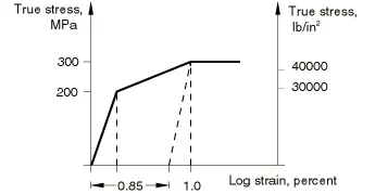
First yield occurs at 200 MPa (29000 lb/in2). The material then hardens to 300 MPa (43511 lb/in2) at one percent strain, after which it is perfectly plastic. Assuming that the Young's modulus is 200000 MPa (29 × 106 lb/in2), the plastic strain at the one percent strain point is .01 − 300/200000=.0085. When the units are newtons and millimeters, the input is
| Yield Stress | Plastic Strain |
|---|---|
| 200. | 0. |
| 300. | .0085 |
Plastic strain values, not total strain values, are used in defining the hardening behavior. Furthermore, the first data pair must correspond with the onset of plasticity (the plastic strain value must be zero in the first pair). These concepts are applicable when hardening data are defined in a tabular form for any of the following plasticity models:
The input required to define hardening is discussed in the referenced sections.
Specifying initial equivalent plastic strains
Initial values of equivalent plastic strain can be specified in Abaqus for elements that use classical metal plasticity or Drucker-Prager plasticity by defining initial hardening conditions . The equivalent plastic strain (output variable PEEQ) then contains the initial value of equivalent plastic strain plus any additional equivalent plastic strain due to plastic straining during the analysis. However, the plastic strain tensor (output variable PE) contains only the amount of straining due to deformation during the analysis.
The simple one-dimensional example shown in illustrates the concept.
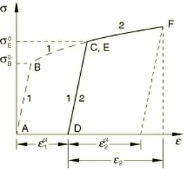
The material is in an annealed configuration at point A; its yield stress is σB0">σ0BσB0. It is then hardened by loading it along the path (A,B,C,D)">(A,B,C,D)(A,B,C,D); the new yield stress is σE0">σ0EσE0. A new analysis that employs the same hardening curve as the first analysis takes this material along the path (D,E,F)">(D,E,F)(D,E,F), starting from point D, by specifying a total strain, ε2">ε2ε2. Plastic strain ε2pl">εpl2ε2pl will result and can be output (for instance) using output variable PE11. To obtain the correct yield stress, σE0">σ0EσE0, the equivalent plastic strain at point E, ε1pl">εpl1ε1pl, should be provided as an initial condition. Likewise, the correct yield stress at point F is obtained from an equivalent plastic strain PEEQ=ε1pl+ε2pl">=εpl1+εpl2=ε1pl+ε2pl.
Plasticity theories
Most materials of engineering interest initially respond elastically. Elastic behavior means that the deformation is fully recoverable: when the load is removed, the specimen returns to its original shape. If the load exceeds some limit (the “yield load”), the deformation is no longer fully recoverable. Some part of the deformation will remain when the load is removed, as, for example, when a paperclip is bent too much or when a billet of metal is rolled or forged in a manufacturing process. Plasticity theories model the material's mechanical response as it undergoes such nonrecoverable deformation in a ductile fashion. The theories have been developed most intensively for metals, but they are also applied to soils, concrete, rock, ice, crushable foam, and so on. These materials behave in very different ways. For example, large values of pure hydrostatic pressure cause very little inelastic deformation in metals, but quite small hydrostatic pressure values may cause a significant, nonrecoverable volume change in a soil sample. Nonetheless, the fundamental concepts of plasticity theories are sufficiently general that models based on these concepts have been developed successfully for a wide range of materials.
Most of the plasticity models in Abaqus are “incremental” theories in which the mechanical strain rate is decomposed into an elastic part and a plastic (inelastic) part. Incremental plasticity models are usually formulated in terms of
-
a yield surface, which generalizes the concept of “yield load” into a test function that can be used to determine if the material responds purely elastically at a particular state of stress, temperature, etc;
-
a flow rule, which defines the inelastic deformation that occurs if the material point is no longer responding purely elastically; and
-
evolution laws that define the hardening—the way in which the yield and/or flow definitions change as inelastic deformation occurs.
Abaqus/Standard also has a “deformation” plasticity model, in which the stress is defined from the total mechanical strain. This is a Ramberg-Osgood mode and is intended primarily for ductile fracture mechanics applications, where fully plastic solutions are often required.
3. Explain Mass, Stiffness & Damping components in the equation of motion
Answer:-
The stiffness load, and constant frequency added mass and damping loads, are calculated using the formulae given below.
All these loads are applied at the unless otherwise stated.
Stiffness load
The specifies how the net weight and buoyancy load (force and moment) on the vessel varies with heave, roll and pitch relative to the vessel in its.Only the heave, roll and pitch components of the matrix are specified; the components for the surge, sway and yaw directions are all zero.
The hydrostatic stiffness matrix, K, encodes how the weight and buoyancy loads on the vessel change due to small changes in the vessel's position and orientation. Two effects contribute to K: the change in load due to the change in the submerged volume of the vessel as it heaves, rolls and pitches (often referred to as waterplane area effects), and the change in moment caused by movement of the vessel's centre of mass and centre of buoyancy as it rolls and pitches (moment arm effects). The hydrostatic stiffness matrices output by most diffraction packages (e.g. WAMIT, AQWA) account for both of these contributions. As stated, the hydrostatic stiffness matrix is only applicable for small changes in the vessel's position and orientation; it is a linearisation of what is, in general, a nonlinear problem. Whilst OrcaFlex cannot account for the waterplane area effects in a nonlinear fashion (since it does not have detailed information about the shape of the vessel hull), it is able to capture the moment arm effects during a simulation by simply applying the weight and buoyancy forces at the instantaneous positions of the centres of mass and buoyancy respectively (under the assumption that the volume of water displaced by the vessel remains constant). To do this, we must subtract the linearised approximation to the moment arm effects from the user's stiffness matrix. This is only possible if vessel's centre of buoyancy has been specified explicitly: if it has instead been input as (~,~,~), meaning that it is at an unspecified position on the same vertical line as the centre of mass, then we do not know the length of the moment arm needed to adjust K. OrcaFlex therefore has two modes of calculation:
Centre of buoyancy unspecified
The net weight and buoyancy load is calculated using the matrix equationl=l0−Kp(1)where
l=[fz,mx,my]T is a column 3-vector containing the heave, roll and pitch components of the net weight + buoyancy load that acts on the vessel. The moments Mx and My are about the vessel x- and y-directions, while the force Fz acts along the diffraction frame z-axis. The superscript T denotes transpose, simply to turn the row-vector written into a column vector.
l0 is the value of l when the vessel. This will be zero if the datum position is a free-floating equilibrium position of the vessel when no other are connected. Otherwise, when the mass of water displaced by the vessel in its datum position is not equal to structural mass of the vessel, l0 will be a pure force acting vertically.
K is the user-specified hydrostatic stiffness matrix.
p is a column 3-vector containing the heave position and roll and pitch angles (in radians) at the reference origin, relative to the user-specified of that reference origin.
So p1=Z coordinate of reference origin−(mean surface Z+datum Z relative to surface). And p2 and p3 are the roll and pitch (in radians) needed to rotate the vessel from its datum heel and trim orientation to its current orientation.
Centre of buoyancy specified
Alternatively, if the centre of buoyancy is given, then the buoyancy load arising from waterplane area effects is calculated froml=−K′p(2)where K′ is the user's stiffness matrix, K, after the removal of the appropriate moment arm contributions. The moment arm contributions are removed by subtracting a term of the form (mwzb−mzg)g from the roll-roll and pitch-pitch components of K, where m is the structural mass of the vessel, mw the mass of displaced water and zb and zg are the vertical distances of the centre of buoyancy and centre of mass above the reference origin when the vessel is in its datum position.
In addition, OrcaFlex applies a weight force vertically at the vessel's centre of massfg=−mg(3)and a buoyancy force vertically at the vessel's centre of buoyancyfb=mwg(4)These two forces are applied by OrcaFlex at every time-step of the simulation, which means that the nonlinear effects of the shift in the moment arm between the centres of mass and buoyancy will be captured precisely. Conversely the change in the buoyancy load associated with the waterplane area effect can only be captured linearly because OrcaFlex has no knowledge of the vessel's geometry above and below the waterline.
Allowing the centre of buoyancy to be specified in this way enables OrcaFlex to model systems where the waterplane area effect is relatively small, e.g. spars. In such a system, allowing for the nonlinear shift in the centre of buoyancy moment arm will result in an accurate buoyancy load even at large angles. However, for some systems where the waterplane area effect is significant, the inconsistency between the linear treatment of the waterplane area effect and the nonlinear treatment of the moment arm may become undesirable at large angles.
Calculation of roll and pitch for hydrostatic stiffness load
For a vessel using calculation mode, a choice is offered for the calculation of the angles provided to hydrostatic stiffness in p. The option named orientation is decomposition. The orientation matrix that describes the rotational offset between the vessel and the vessel is converted into Euler angles, and those roll and pitch angles are used in p.
The option named subtraction is to subtract the vessel type angles from the instantaneous roll and pitch angles of the primary frame. The rotational offset between the vessel primary frame and the global axes is converted into Euler angles, and then the datum angles are subtracted from these.
These two options will give the same results for a vessel type with zero datum trim angle. For cases with significant non-zero datum trim, we recommend the orientation calculation method, because we believe it to be more rigorous.
Added mass and damping loads
The theory here gives details of the added mass and damping loads when using the constant The calculation for frequency-dependent added mass and damping loads is more complex, and is described in but the units given below apply in both cases.
Damping load
When using the constant the damping load is equal to −Dv, where D is the specified constant and v is the (6 degree of freedom) vector of vessel velocity and angular velocity relative to the earth at the specified
The damping load is calculated from the matrix equationl=−Dv(5)where
l=[fx,fy,fz,mx,my,mz]T is the column 6-vector containing the components, in the vessel directions, of the damping force (fx,fy,fz) and moment (mx,my,mz) that act on the vessel
D is the user-specified damping matrix.
v=[vx,vy,vz,ωx,ωy,ωz]T is the column 6-vector containing the components, in the vessel directions, of the velocity (vx,vy,vz) at the specified and the angular velocity (ωx,ωy,ωz) of the vessel, relative to earth.
When using the constant the added mass load calculation is analogous to the described above.
The added mass and damping load (force and moment) at the is therefore equal to −Maa, where Ma is the given and a is the column 6-vector containing the components, in the vessel directions, of the vessel translational and angular acceleration relative to earth
The angular accelerations are expressed in radians/T2, so the units of the 3×3 blocks of the added mass matrix are[MMLMLML2]where M, L and T denote the of mass, length and time, respectively.
4. Provide relationship between Natural period (Tn) & Natural frequency (f) and provide their definitions
Answer:-
Natural Period Tn of a building is the time taken by it to undergo one complete cycle of oscillation. It is an inherent property of a building controlled by its mass m and stiffness k. These three quantities are related by its units are seconds (s)
Natural period:
- The natural period of a building is simply a time taken by it to undergo one complete cycle of oscillation.
- The natural period is one of the properties or building which is controlled by mass and stiffness.
- Formula to find out natural period is,
Tn =2π√(m/k) where,
Tn is a natural period of building.
m is mass
k is stiffness
Reciprocal of the natural period of a building is nothing but the natural frequency and its unit is Hertz(Hz)
imply put, the time period of a building is it’s natural period of oscillation when subjected to ground shaking in the event of an earthquake.
The building is modelled to be under harmonic oscillation and the time period is calculated in a similar way as in harmonic oscillation
T = 2π√(k/m)
where k is the total stiffness and m is the total mass.
k is calculated as the sum of the lateral stiffness of all stiffness providing and moment resisting vertical members (colomns, moment resisting frames, sheer walls, etc.) m is calculated as the sum of masses of all members on the storey.
Natural frequency (f) =√stiffness/√Mass of structure.
- Take the case of a very tall building which is susceptible to damage whan earthquake occur will have higher group and hence lower natural frequency.
- Thereby, it is desirable to have higher natural frequencies. Also, at low natural frequencies, the structure can resonate easier and hence lead to amplification.
- I do not know enough about building dynamics to comment about this mathematically, but this is a plausible argument.
A building’s natural frequency (n) is simply the inverse of the fundamental period (T), and, for flexible and dynamically sensitive buildings and other structures, this natural frequency is used in the calculation of the Gust Factor. The ASCE 7 standard specifies that buildings are considered “flexible” if they have a fundamental period greater than 1 second. Tall building or moment-frame buildings tend to be more flexible than others, so these code criteria can have a significant impact on their design and their construction costs. And engineering judgement is required when the natural frequency/fundamental period of the structure is near 1.0 and note that the nonbuilding structure or components with the fundamental period less than 0.06 s shall be considered a rigid element.
5. Explain in detail about Response spectrum & its Graph
Answer:-
A response spectrum is a graphical plot of the frequency of an oscillator and its damping. The response spectrum plot represents the peak or steady-state response (velocity, displacement, or acceleration) of a series of oscillators of varying natural frequency. In vibration analysis of any system, the response spectrum is very useful as the resulting plot can provide the response of any linear system with respect to its natural frequency. The response spectrum finds its usage in interpreting seismic or earthquake events and slug flow events.
Response Spectrum Analysis is a scientific method for estimating the structural response of dynamic vibration events. To perform the response spectrum analysis, the first job is to define the response spectrum of the system. In this article, we will explore the basics of the response spectrum and learn the steps for performing seismic/earthquake analysis using the response spectrum analysis method.
Response Spectrum Analysis Method
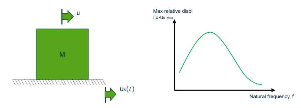
Response spectrum plot gives the maximum response (that maybe maximum displacement, maximum velocity, maximum acceleration, or any other parameter of interest) to the natural frequency (or natural period) subjected to specified excitation for linear single degree of freedom system oscillators. These plots are subjected to specific damping and it changes as damping changes. Refer to Fig. 1 shown below:
Parameters affecting Response Spectra
The response spectral values are dependent on various factors like,
- Soil condition
- Energy release mechanism
- Damping in the system
- Epicentral distance
- Focal depth
- Richter magnitude
- Time period of the system
Construction of Response Spectrum Plot
The construction of Response Spectrum requires the solution of a single degree of freedom systems, for a sequence of natural frequency values and damping ratio in the range of interest. Every solution provides only one point (with the maximum value) of the response spectrum. All of these maximum response values are plotted against natural frequency to construct a single response spectrum.
Since a large number of systems must be analyzed in order to fully plot each response spectrum, the task is lengthy and time-consuming. But once these curves are constructed and available for the excitation of interest, the analysis for the design of structure subjected to dynamic loading is reduced to a very simple calculation of the natural frequency of the system and the use of response spectrum to calculate the maximum response.
So, let’s look at a simplified example of how we can get a response spectrum plot for a specific area of the region.