Steady Vs Unsteady flow over a cylinder

TO SIMULATE THE FLOW OVER THE CYLINDER AND EXAMINING THE PHENOMENON OF KARMAN VORTEX STREET

Aim:

To simulate the flow over the cylinder and examining the phenomenon of Karman vortex street.

Introduction:

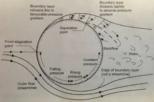
The von Kármán vortex street is a direct result of boundary layer separation over bluff bodies. Immersed in fluid flow, anybody of finite thickness will force the surrounding fluid to flow in curved streamlines around it. Towards the leading edge this causes the flow to speed up in order to balance the centripetal forces created by the curved stream lines. This creates a region of falling fluid pressure, also called a favourable pressure gradient. Further along the body, where the streamlines straighten out, the opposite occurs and the fluid flows into a region of rising pressure, an adverse pressure gradient. The increasing pressure gradient pushes against the flow and causes the slowest parts of the flow, those immediately adjacent to the surface, to reverse direction. At this point the boundary layer has separated from the body and the combination of flow in two directions induces a wake of turbulent vortices.

Theory:

Consider the flow past an infinitely long cylinder protruding out of your screen (as shown in the figure above). For very low Reynolds number flow (Re < 10) the inertial forces are negligible and the streamlines connect smoothly behind the cylinder. As the Reynolds number is increased into the range of Re = 10-40 (by, for example, increasing the free stream velocity or by decreasing the viscosity), the boundary layer separates symmetrically from either side of the cylinder, and two eddies form that rotate in opposite directions. These eddies remain fixed and do not “peel away” from the cylinder. Behind the vortices the flow from either side re-joins and the size of the wake is limited to a small region behind the cylinder. As the Reynolds number is further increased into the region Re > 40, the symmetric eddy formation is broken and two asymmetric vortices form. Such an instability is known as a symmetry-breaking bifurcation in stability theory and the ensuing asymmetric vortices undergo periodic oscillations by constantly interchanging their position with respect to the cylinder. At a specific critical value of Reynolds number (Re ~ 100) the eddies start to peel away, alternately from either side of the cylinder, and are then washed downstream.

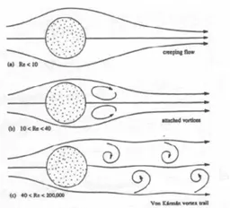
This condition of alternately shedding vortices from the sides of the cylinder is known as the von Kármán vortex street.

Practical application:

There are two very important locations on an aircraft wing:
1. The centre of pressure, i.e. an idealised point of the wing where the lift can be assumed to act as a point load.
2. The shear centre, i.e. the point of any structural cross-section through which a point load must act to cause pure bending and no twisting.

The problem is that the centre of pressure and shear centre are very rarely coincident, and so the aerodynamic lift forces will typically not only bend a wing but also cause it to twist. Twisting in a manner that forces the leading edge upwards increases the angle of attack and thereby increases the lift force. This increased lift force produces more twisting, which produces more lift, and so on. This phenomenon is known as divergence and can cause a wing to twist-off the fuselage.

Modelling approach:

Open the Ansys workbench to create geometry, mesh and for simulating the problem.

Drag the fluid flow (fluent) to the screen to use the options.

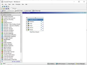
Ansys workbench

Solver and Modelling approach:

• Ø Step 1: Creating Geometry

Double click on the geometry to open the space claim window, by using the tools in the space claim create a geometry which resembles a cylinder on a plane.

• Ø Step 2: Meshing:

The imported geometry is meshed to the required mesh size focusing more on the boundary around the cylinder since our entire physics of the problem depends on the cylinder boundary.

The naming of the boundaries is also done here for future reference.

• Ø Step 3: Setup

By double clicking the setup option, the fluent will open and any errors regarding geometry or meshing will be shown by the console window.

Even the running errors during the simulation can also be seen in the console window.

We are going to setup the required physics by selecting required

• Type of flow
• Materials and its properties
• Boundary conditions and all the required properties for the study.

• Ø Step 4: Initializing and running:

Once the entire physics for the problem was uploaded and checked, click on definitions to see the required outputs you are interested in (like velocity distribution, pressure distribution etc.)

Now initialize the solution to give the software a beginning value to start the iteration.

For running,

If it is a steady flow, give the number of iterations

If it is a transient case, give required number of time steps and size of time step and click on calculate for running.

• Ø Step 5: Creating contour plots and animations:

In order to generate the contour plots of velocity and pressure for analyses, click on the results

Go to contours select new and give the required information about the contour like if we want plot a velocity contour select velocity in the contours of column select all the surfaces and click on compute and then save and display.

For animation:

In the solutions at activities click on create and then solution animations give the necessary details like name, at how many iterations software has to record and animation object and click ok.

• Ø Step 6: checking and Analyzing the results:

Once the results are obtained it is very important to understand and check the results by analyzing whether the results fit to the actual physics of the problem.

Once we are satisfied with the results then proceed with the analyses of results in order to draw some conclusions.

If not satisfied, we need to go back and look into the geometry, meshing, setup and do some required and valid modifications to proceed further.

Preprocessing and solver settings:

Geometry:

Since the simulation is regarding the flow over a cylinder, we need to create a domain which contains a cylinder, inlet and outlet.

In order to create such geometry, initially set the units of length in meters by changing the space claim settings.

Now create a circle of required diameter, and a surface with inlet and outlet distances as specified.

Circle diameter: 2 meters

Inlet distance from center of circle: 20

Outlet distance from center of circle: 40

Now create a plane on the surface by using the pull tool, and delete the circle from it because it doesn’t belong to the plane.

Also delete all the construction lines used for the geometry in order to avoid these lines to involve in the geometry.

Ensure that the center of circle lies exactly at the center of plane as it is important when we are creating a monitor point

Now our geometry is ready for the meshing.

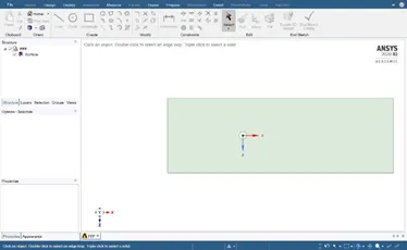
Geometry for flow over cylinder

Meshing:

Since our geometry is simple 2D plane triangular mesh will give us good results and also choosing triangular mesh will reduce our simulation time.

But the cylinder boundary is an important consideration in our study because our fluid is flowing on the walls of the cylinder, so we need to take an appropriate care on the meshing around the boundaries.

In order to generate a smooth curve around the edge of the cylinder, use the sizing option in order to increase the number of divisions allocated for that edge (increase the divisions to 36).

In order to make the curve more fitting to our physics, use the inflation method by giving first layer height as 0.005 and number of layers as 6 (values can also be changed according to requirement).

Meshing Requirements:

Element size: 0.25 (after checking different mesh sizes, this size is showing good vortex formation)

Sizing type: Number of divisions (36)

Inflation option: first layer thickness

First layer height: 0.005

Number of layers: 10

Name the inlet, outlet, cylinder wall and other two edges for future reference.

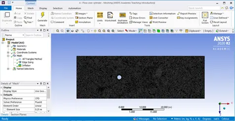
Meshing

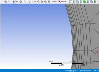
Cylinder edge after sizing and inflation

Setup:

Look for any errors in the console window, if no then look whether the mesh is correctly loaded and the boundaries are updated.

If everything is fine, then go for mesh check, if console window doesn’t show any error proceed to setup.

Give the general settings like type and time of flow, velocity formulation.

Now by going into the physics setup, we need to create our material according to our requirement by copying one of the fluids from the fluid database and specifying required properties to get the appropriate Reynolds number (by specifying density, velocity, dynamic viscosity of fluid).

Select the laminar condition as we are dealing with the Reynolds numbers of less than 2*10^5.

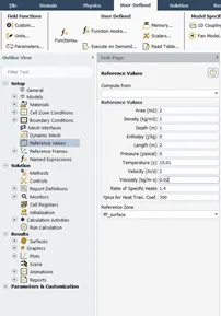
Properties of fluid for Re=100

Select the inlet boundary condition with velocity of fluid at the inlet, and atmospheric pressure at the outlet, no slip boundary condition for the wall and symmetry boundary condition for other two edges.

Select a monitor point at an appropriate position, for calculating the vortex average method for the flow, now plot and report a file for velocity vortex average at the monitor point.

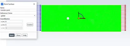
Monitor point setup

Reports and Definitions setup:

We are looking at three different quantities for analyzing the flow by going into solution setup and creating reports and plots.

1. Surface report for vortex average of velocity
2. Force report for coefficient of lift
3. Force report for coefficient of drag

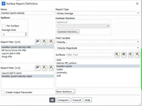
Surface report for velocity at monitor point

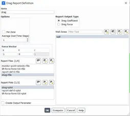
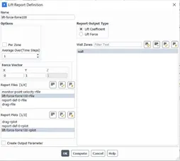
Drag force report setup lift force report setup

In the residuals setup uncheck all the convergence criteria because we need to run the iterations completely to get proper results of the problem.

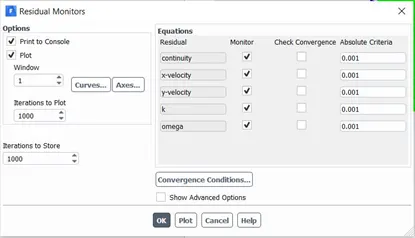
Residual setup

Setting up contours:

In order to look at the flow behavior, it is important to create a contour with respect to velocity and pressure.

So, create a contour in the results setup for velocity and pressure by giving contour name, variable and selecting all the surfaces.

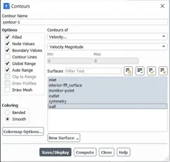
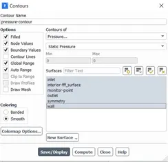
Velocity Contour setup pressure contour setup

Animation setup:

To look at the flow behavior in a continuous motion to get a clear idea of flow behavior and vortex formations, it is important to create an animation profile.

For creating an animation go to solution setup, in the activities click on create and then solution animation, give the name, animation object and after how many each iterations we need to look at animation.

Results:

The problem contains two parts:

Part 1:

For Re=100

1. Simulating the steady flow
2. Simulating the transient flow and calculating Strouhal number for both cases.

Part 2:

For steady flow:

1. Calculating the coefficient of drag and lift over a cylinder by setting the Reynolds number to 10,100,1000,10000 & 100000.
2. Discussing the effect of Reynolds number on the coefficient of drag for each case.

Simulation of steady flow for Re=100

We are going to analyze the results based on the

• Residuals (mainly to check the convergence of the solution).
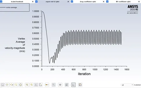
• Vortex average plot of velocity (in order to check the vortex formation existence).
• Velocity contour plot (to physically experience and analyze the formation of vortex)
• Residual plot:

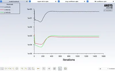
Residuals plot (it is very clear that convergence happened after 400 iterations)

Vortex average plot for velocity:

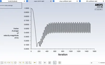
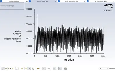
The fluctuations in the graph indicates the formation of vertices at the monitor point that we have defined, after seeing this plot we can come to a conclusion that formation of Karman vortex has happened in the flow.

Velocity contour plot:

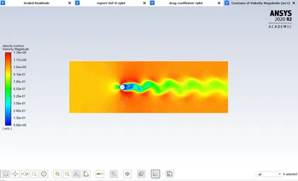
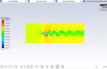
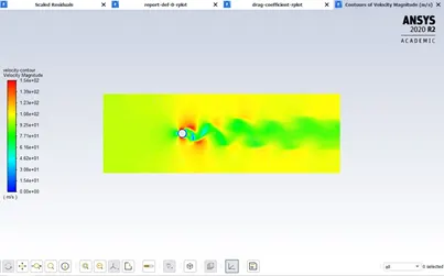
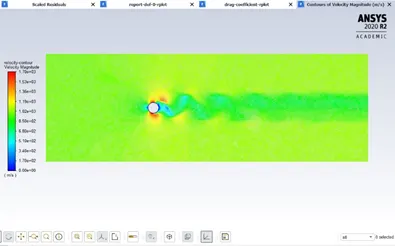
we can very clearly see that the flow after passing the cylinder has created eddies and there was a fluctuation of velocity behind the cylinder.

Coefficient of drag and lift:

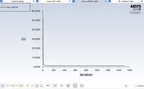
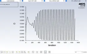
Cd=1.31858 (obtained from console window) Cl=0.0622

Calculation of Strouhal number:

In order to get the value of Strouhal number go to plots in the outline view and then click on FFT, import coefficient of lift file, select X-axis as Strouhal number and Y-axis as magnitude of coefficient of lift and then plot FFT.

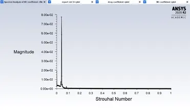
Also write a FFT file to clearly note the Strouhal number, by taking the peak magnitude value of coefficient of lift as reference identify the Strouhal number in the write FFT file.

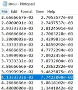
The value of Strouhal number for steady flow with Re=100 is: 0.04133

Simulation of Transient flow for Re=100

Residual plot:

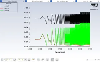
Around after 7500 iterations the solution has been converged.

Vortex average plot for velocity:

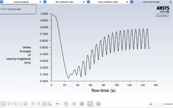
There is a clear fluctuation in the graph which clearly indicates the formations of Karman vorticity in the flow.

Velocity Contour plot:

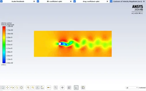
Clear indication of formation of eddies and vorticity once the flow past the cylinder.

Coefficient of drag and lift:

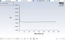
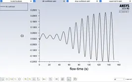
Cd=1.3458 Cl=-0.18386

Strouhal number:

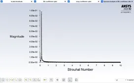
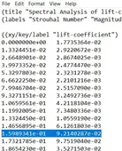
The spectral value is: 0.159

Part 2:

Calculation of coefficient of drag and lift for different values of Reynolds number:

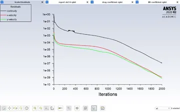
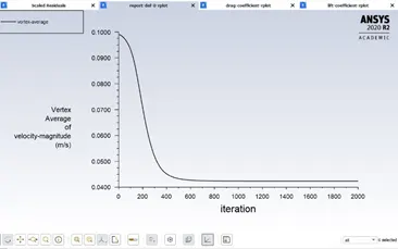
For Re=10:

Residuals plot:

Vortex average of velocity :

Coefficient of Drag and Lift:

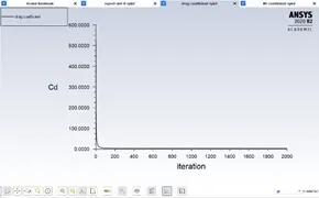
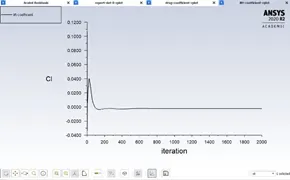
Cd=3.32445 Cl=-0.0022

Velocity contour plot:

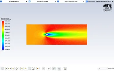
• Clearly there is no Karman vortex formation for Re=10

For Re=100:

• Residual plot:

Vortex average plot for velocity:

Coefficient of drag and lift:

Cd=1.31858 Cl=0.0622

Velocity contour plot:

For Re=1000:

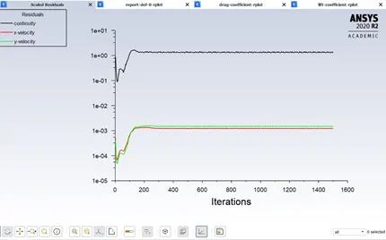
Residual plot:

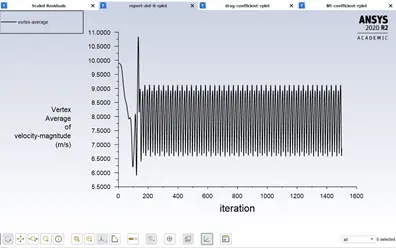
Vortex average velocity:

Coefficient of Drag and lift:

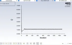
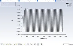
Cd=1.090178 Cl=0.16065

Velocity contour plot:

For Re=10,000:

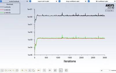
Residuals plot:

Vortex average of velocity:

Coefficient of Drag and Lift:

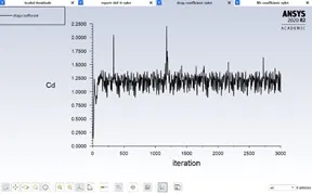
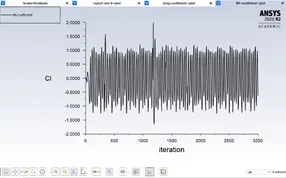
Cd=0.9834 Cl=-0.6292

Velocity contour plot:

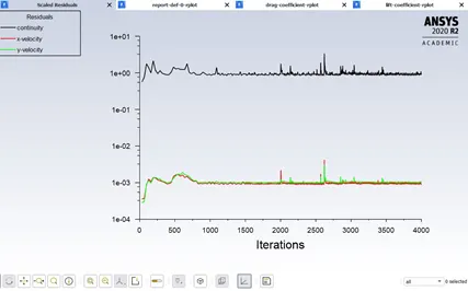
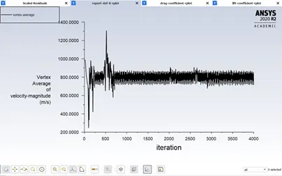
For Re=1,00,000:

Residual plot:

Vortex average of velocity:

Coefficient of Drag and Lift:

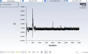
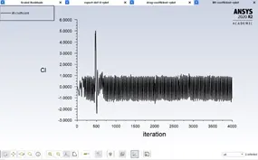
Cd=0.88513 Cl=-1.0514

Velocity contour plot:

Let us tabulate the values of coefficient of Drag and Lift for different values of Reynolds number

Reynolds number	Coefficient of Drag Cd	Coefficient of Lift Cl
10	3.32445	-0.0022
100	1.31858	0.0622
1000	1.090178	0.16065
10,000	0.9834	-0.6292
1,00,000	0.88513	-1.0514

Effect of Reynolds number on the Coefficient of Drag:

• Clearly as Reynolds number increases, value of Coefficient of Drag is decreasing, initially the decrease of Cd value is more but at high Reynolds number the decrease in value is relatively very low.
• The value of coefficient of lift is fluctuating from -1 to +1 for different Reynolds number.
• As the Reynold number is increasing, the fluctuations in the values of Cd and Cl is increasing. So, it takes a greater number of iterations to get a stable value for Cd and Cl as the Re increases.

Preferred material:

For basics of undersatnding karman vortex phenomenon:

refer: https://aerospaceengineeringblog.com/the-von-karman-vortex-street-and-tacoma-narrows-disaster/

for literature survey:

Refer:

https://doi.org/10.1016/j.apm.2008.01.017