Mixing efficiency

                                 ANALYSIS OF T-JOINT MIXING EFFEICIENCY USING ANSYS INFLUENT

Aim:

To set up steady-state simulations to compare the mixing effectiveness in T joint when hot inlet temperature is 36˚C & the Cold inlet is at 19˚C.

Introduction:

Being of importance for turbulent and thermal mixing and consequently for thermal striping and thermal fatigue problems in nuclear power plants, thermal mixing phenomena have been investigated. 

Here we are using the case of commercial application of T mix for Refrigeration and Air conditioning purpose where there was ca chilled air flow at 19C for my comfort i wanted to change the outlet air temperature for this we are creating a another flow through the inlet 36C using T joint so that mixing of flow takes place by adjusting the flow rate we would get the required flow at the outlet of the Tmix which would be connected to refrigerating space to get our condition fulfilled.

Material: air (fluid)

Property                                Units                Method                Value(s)
---------------------------------------------------------------
Density                                  kg/m3              constant                 1.225
Cp(Specific Heat)                    j/kg-k              constant               1006.43
Thermal Conductivity              w/m-k              constant                0.0242
Viscosity                                kg/m-s             constant             1.7894e-05
Molecular Weight                    kg/kmol            constant               28.966
Thermal Expansion Coefficient   1/k                constant                   0
Speed of Sound                       m/s                  none                      #f

Material: aluminium (solid)

Property                               Units                 Method                 Value(s)
---------------------------------------------------
Density                               kg/m3               constant                  2719
Cp (Specific Heat)                j/kg-k                constant                  871
Thermal Conductivity           w/m-k                constant                 202.4

Theory:

A tee joint is a connection of two members approximately perpendicular to one another, forming two right angles similar to the letter T. This is a result of one member being connected between the two ends of the other. It differs from a corner joint consisting of a single right angle formed by two members each connected to the other at one end. 

This connector may be used to direct the flow of fluid in one direction or the other, to divide it in two directions, or to combine flow from two streams into a single stream. A valve may be used to control the flow of fluid through the joint.

Turbulent mixing of fluid of different temperature in T-junction geometries became significantly important in the field of nuclear reactor safety, since it can lead to highly transient temperature fluctuations at the adjacent pipe walls, cyclic thermal stresses in the pipe walls and consequently to thermal fatigue and failure of the pipeline.

Applications of T joint:

Residential, commercial, and industrial construction of things such as buildings and bridges rely heavily on tee joints to connect structural members.

Ventilation is another application in which tee joints may be used. Where liquids or gases are conveyed through a tee joint, proper sealing of the joint is particularly important to prevent the material from leaking out at any of the points of connection.

software used:

ANSYS FLUENT 2020 R2

Objectives:

• To consider the effects of velocity and length on mixing efficiency.
• To compare k-epsilon and k-omega SST model on mixing problem.
• To perform mesh independent study.

 Solving and Modelling approach:

step 1:

open Ansys workbench and drag fluid flow(fluent) into the screen to access the options.

                                      fig(i) workbench

step 2:

Double click on the geometry to open the space claim, after opening the space claim upload the model that we have to work on.

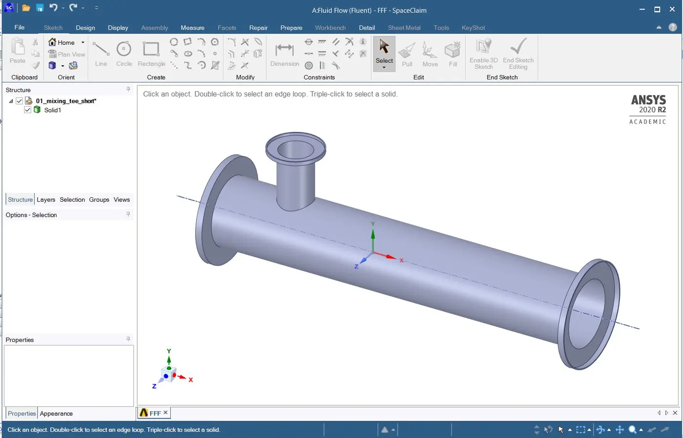
                                    fig(ii) space claim solid model

As we are interested only on the fluid volume that is only those surfaces with which our fluid is interacting, so using volume extract option, by selecting edges option select fluid volume edges  and click ok, immediately we can see a volume on our working tree.

Hide the solid model by unchecking the solid model box to have a look at our fluid volume. 

To get rid of involvement of solid in our study, right click on the solid choose suppress for physics, by doing so our solid willnot involve in meshing and simulation.

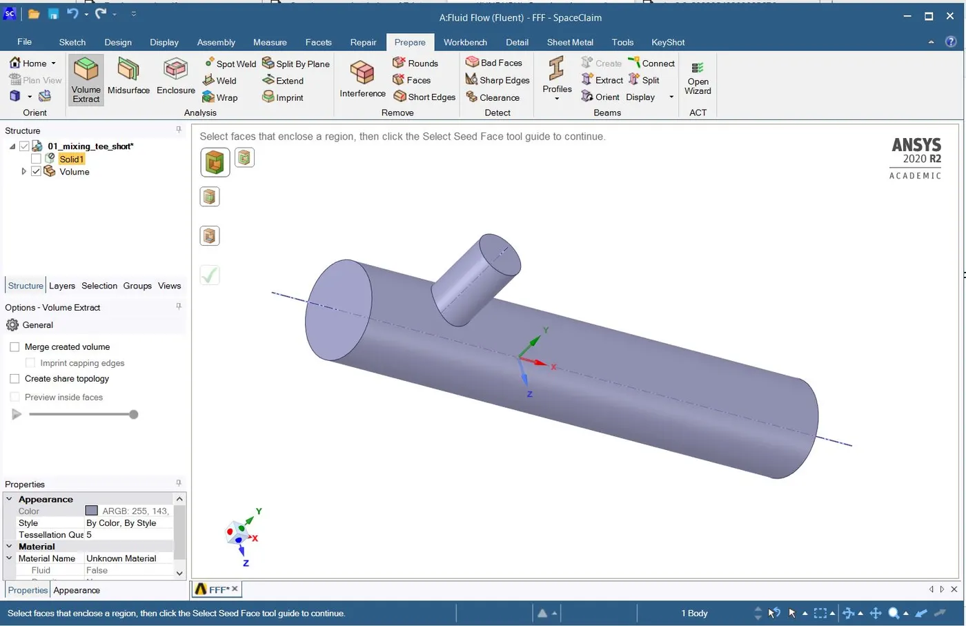
                                          fig(iii) space claim fluid volume

close the space claim window and the work will be automatically saved.

step 3:

Double click on the mesh in the fluid flow(fluent) drag box, mesh window will be opened with the model we created.

Name the boundaries for future reference by selecting the faces (ctrl+F) and naming them(N).

To create the mesh, right click on mesh in the tree diagram and click on generate mesh, mesh will be generared with default meshing size.

We can change the mesh size by clicking on element size and changing the default size.

 

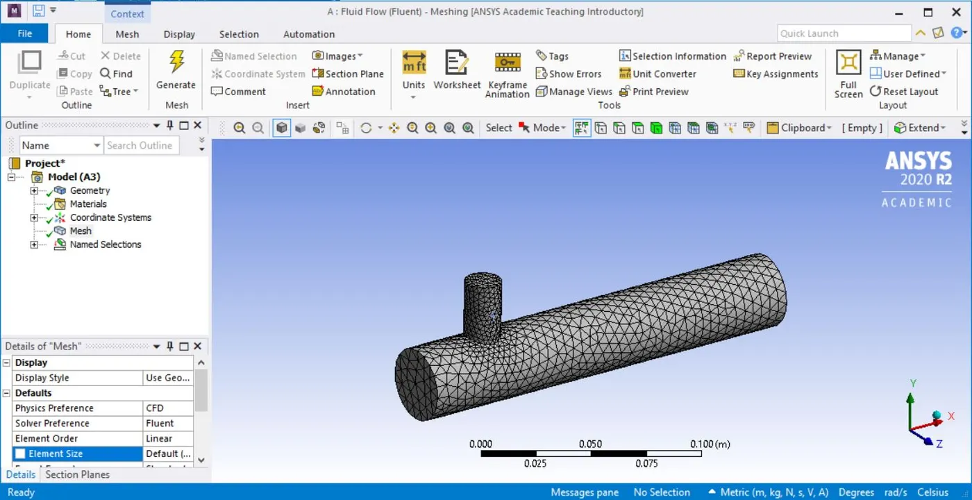
                                                       fig(iv) mesh generation

we can create sectional plane if we want to analyse the behaviour of fluid at different sections or for checking the mesh at different sections, by clicking on section plane and dragging the pointer along the plane which we want to cut.

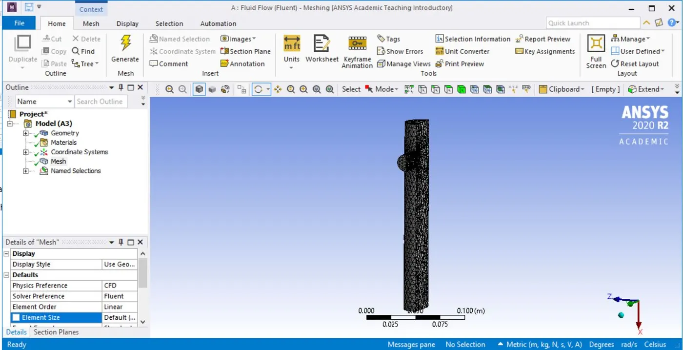
                                                              fig(v) section plane

step 4:

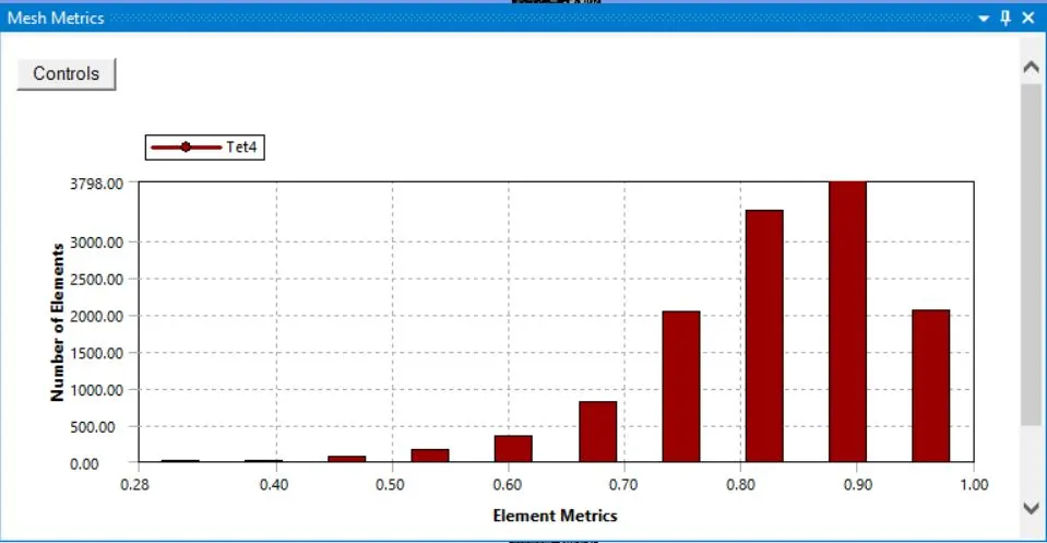
To check the quality of mesh, double click on quality in tree diagram and in mesh metric go to element quality and if our quality is more than 5% then it was a good mesh otherwise go for mesh refinement.

                                                  fig(vi) mesh quality

close the mesh window.

step 5:

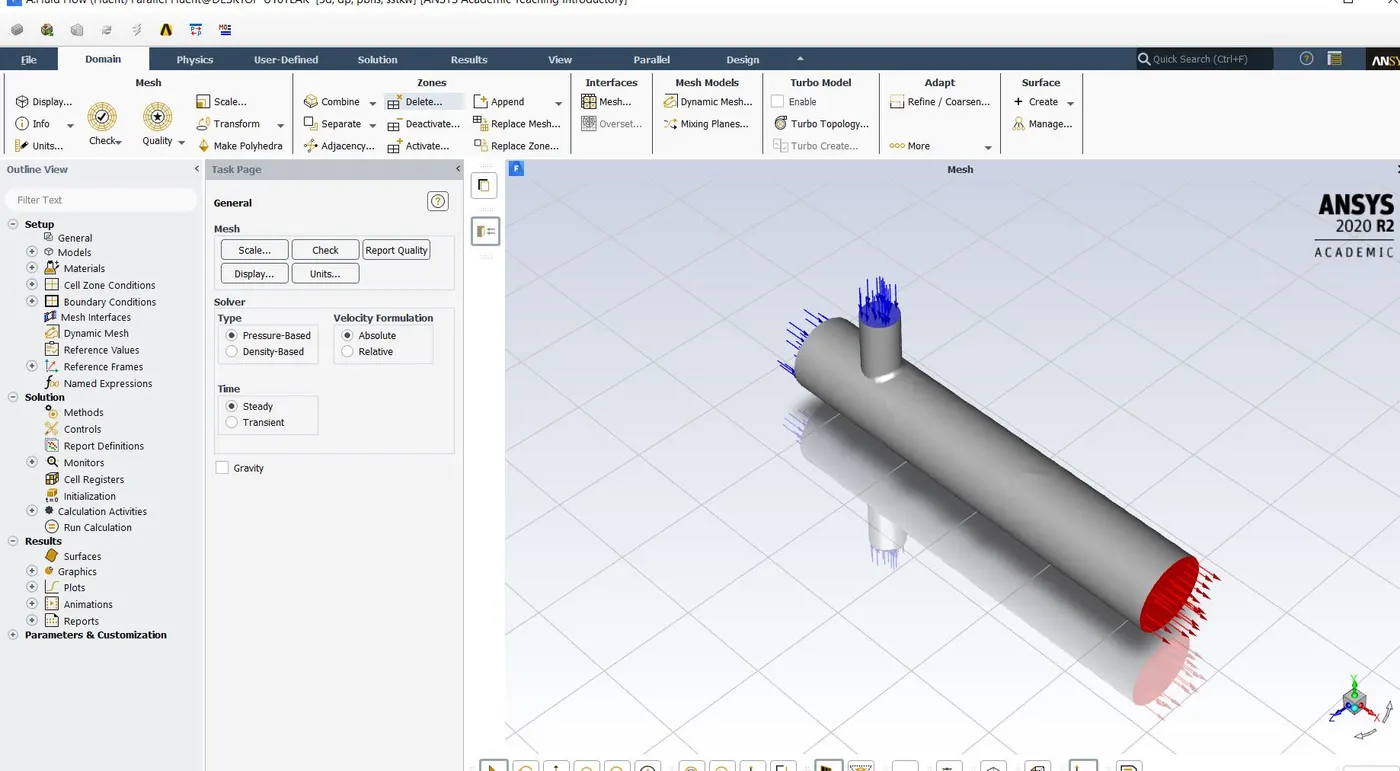
Now open the setup window by double clicking on it in workbench, check the quality of mesh, setup the physics, add material and assign the boundary conditions.

After setting up everything, give the details of outputs which we want to see at the end of solving by going to solving clicking on definitions.

Before calculating the results software requires initial value to start the iteration, so click on initialise to setup initial value for iterations.

Now run the calculations by giving the number of iterations you want the software to perform.

step 6:

After checking the results close the setup window and open the result window by double clicking on results window.

Click on the boundaries in the tree diagram we want to see.

Double click on the wall, click on the render and increase transparency to have a look inside the wall for understanding the fluid behaviour.

Now create planes and lines to analyse by clicking on the insert and then location.

We can also create charts and stream lines for better analyses of the flow.

Problem Definition:

Coming to the problem we need to handle two cases with sub-cases as follows:

Case: 1 T- mixing in short tube      

Sub-case: 1

Hot velocity = 3 m/s                           

Momentum ratio = 2                          

Cold velocity = 6 m/s      

Sub-case: 2

 Hot velocity = 3 m/s                        

 Momentum ratio = 4                          

 Cold velocity = 12 m/s

 Case: 2 T- mixing in long tube   

 Sub-case: 1

Hot velocity = 3 m/s                          

Momentum ratio = 2                          

Cold velocity = 6 m/s      

 Sub-case: 2

Hot velocity = 3 m/s                        

Momentum ratio = 4                          

Cold velocity = 12 m/s

Case: 1 T- mixing in short tube  

Geometry:

we require a solid model of T-section which is having two inlets for sending two streams of different temperature and velocity to analyse outlet behaviour  of existing stream.

The uploaded solid model is prepared in such a way that only fluid volume present in the model.

                                                                         

                       space claim solid model                                                                                      space claim fluid volume                                                                                                 

Meshing: 

As our model is simple geometry, default meshing will be sufficient to get good results as it is giving minimum 28% of quality mesh for this geometry.

Meanwhile name the boundary conditions, for future reference(in this case inlet-x, inlet-y, walls, outlet-x).

                                                                                                                                                                                                                      Generated mesh                                                                                              Mesh quality 

Since the flow is steady, pressure based and absolute velocity formula click on these options in the general setting before proceeding.

In setting up physics, give boundary conditions of inlet-x with velocity 3m/s and temperature 36˚C and inlet-y with velocity 6m/s and temperature 19˚C and since our flow can be turbulent select viscous flow and k-epsilon residual method for analysis.

Mark the energy checkbox as we are dealing with the temperature.

Inorder to know the area weighted avverage value and standard deviation of temperature, give the definitions in the solution section accordingly.

Initialise the values and start the iterations to see the results.

    

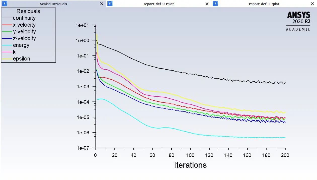
                Residual values for T-short mr=2 and k-epsilon

    

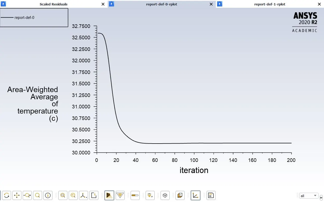
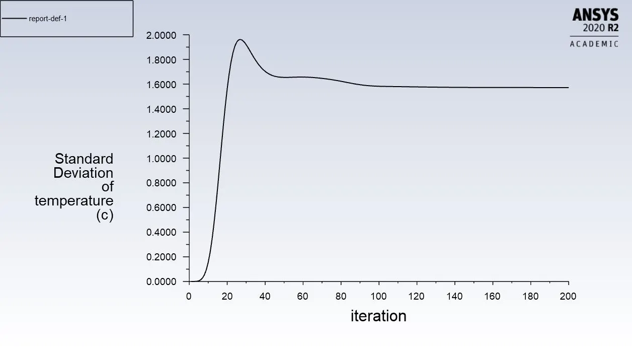
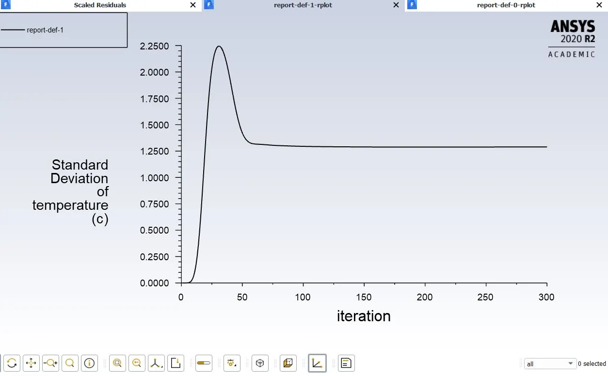
          Area weighted average of temperature  for k-epsilon                                 Standard deviation of temperature for k-epsilon

It is very clear from the graphs that area weighted temperature at the outlet is 30.25˚C and standard deviation in this approach is  1.6.

For momentum ratio=2, using k-omega SST method

With the same setup if we choose  k-omega SST method as our turbulence model the following results are obtained.

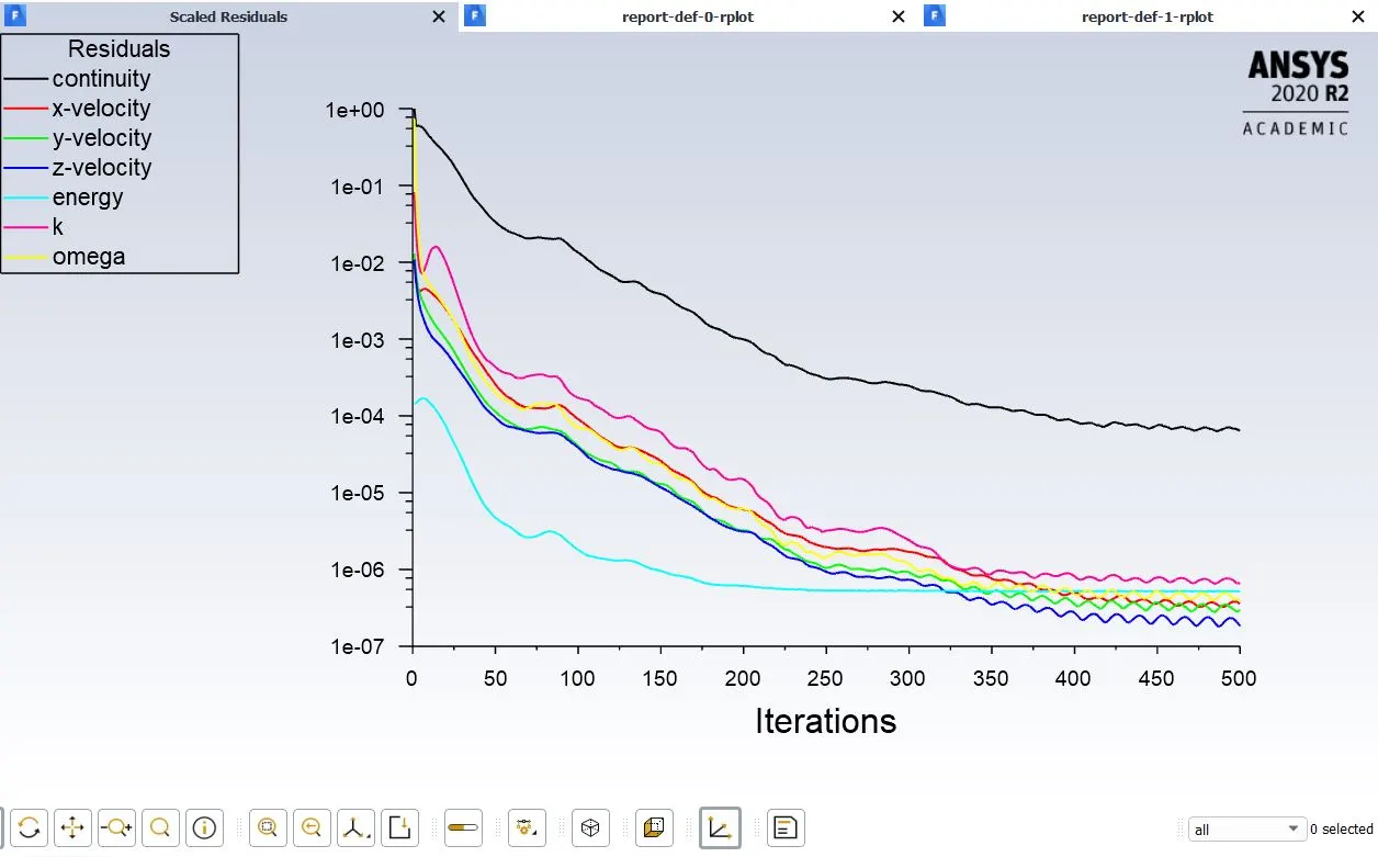
                     Residual values for T-short mr=2 and k-omega

                                     

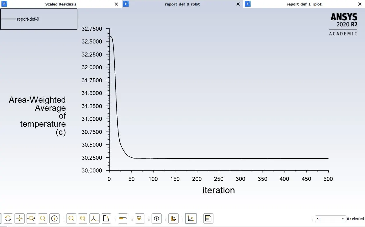
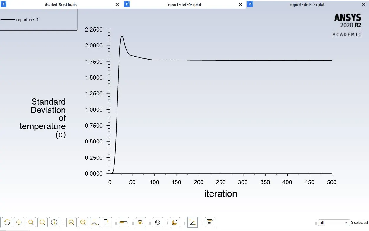
Area weighted average of temperature  for k-omega                            Standard deviation of temperature for k-omega

we can observe that there is no much difference in the area weighted average value but the standard deviation of temperature has increased from 1.6 to 1.75.

So it is evident that k-epsilon has less standard deviation than k-omega so we can proceed further with the k-epsilon residual method. 

Results:

For momentum ratio=2, using k-epsilon residual method:

Temperature along the plane:

                                              

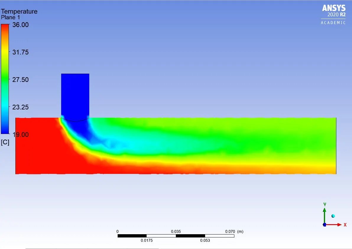
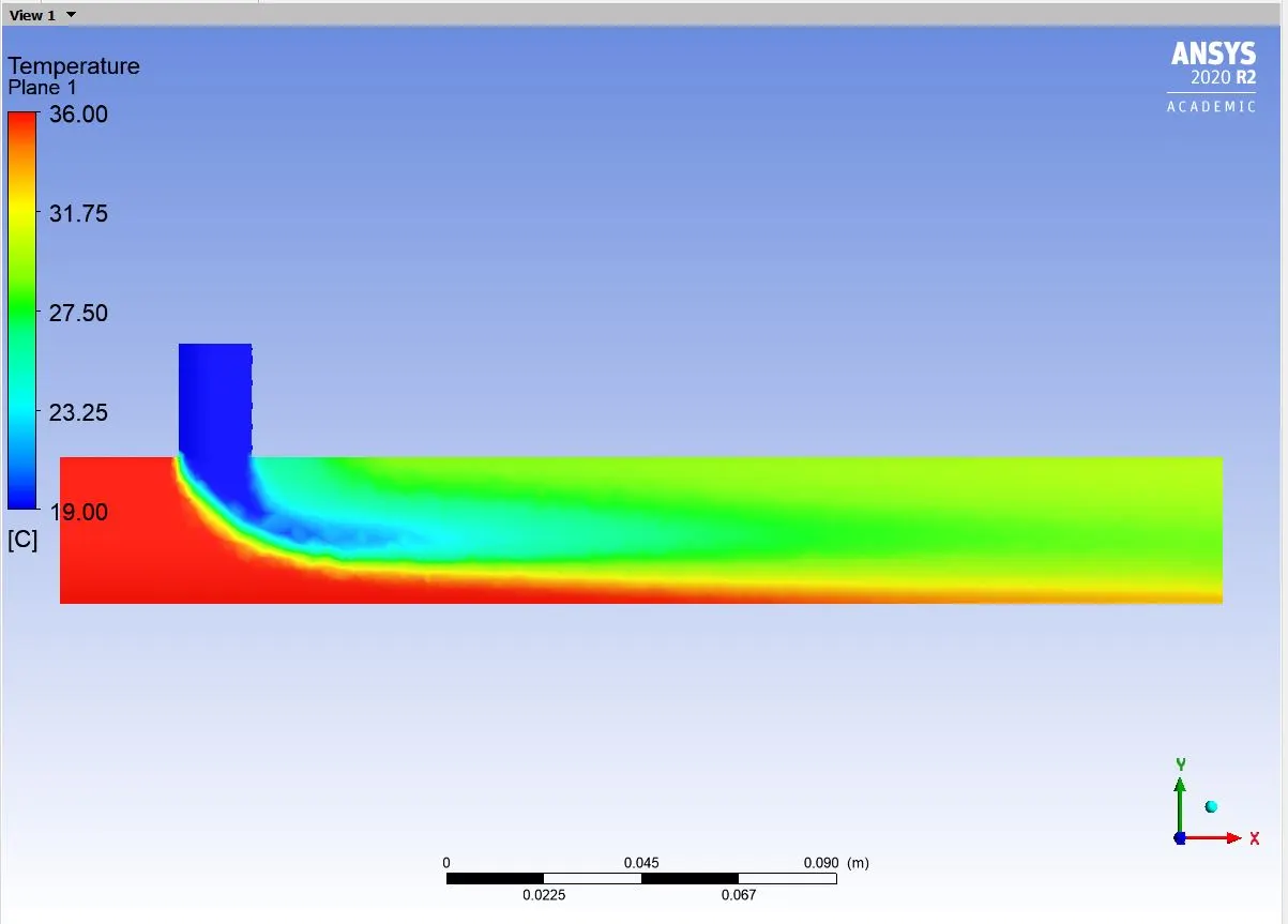
                                           Temperature contour plot along the plane for Tshort(Mr=2,K-epsilon method) 

                                                  

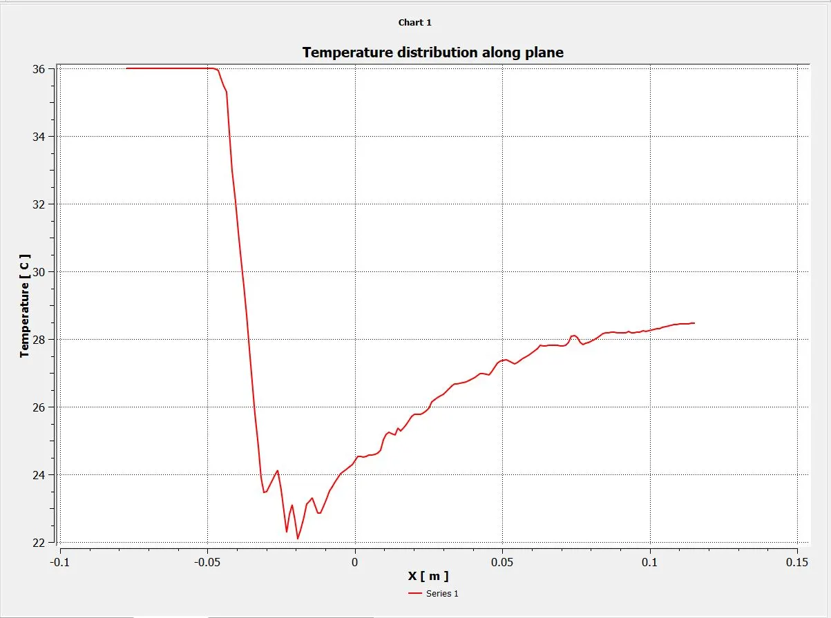
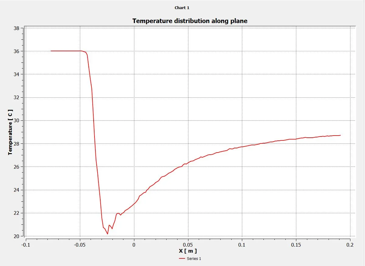
                                              Temperature line plot along the plane for Tshort(Mr=2,K-epsilon method) 

From the two plots we can clearly observe that at the junction of mixing the temperature drops suddenly because of entry of cold fluid and as the mixing process going on along the length of the pipe the temperature starts increasing and reaching a value close to 30˚C at the end.

Temperature across the plane: 

                                                                                                         

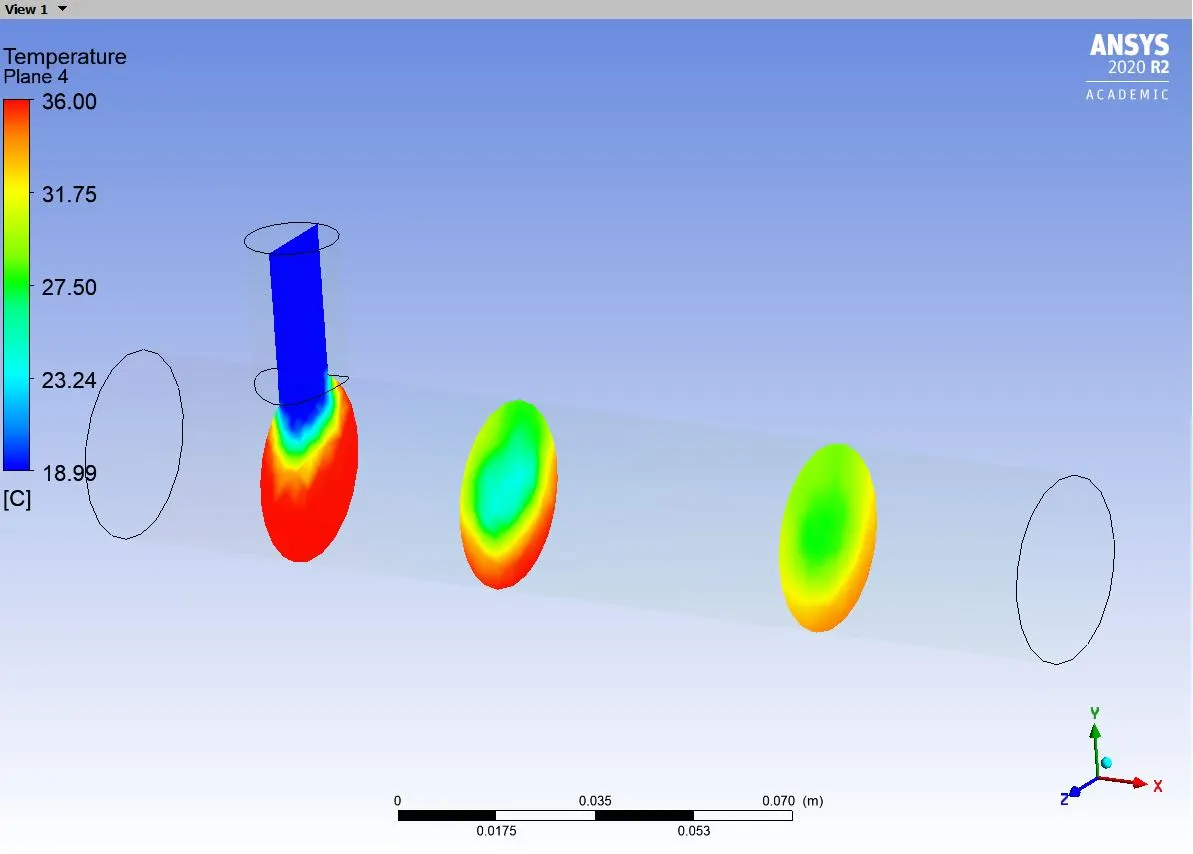
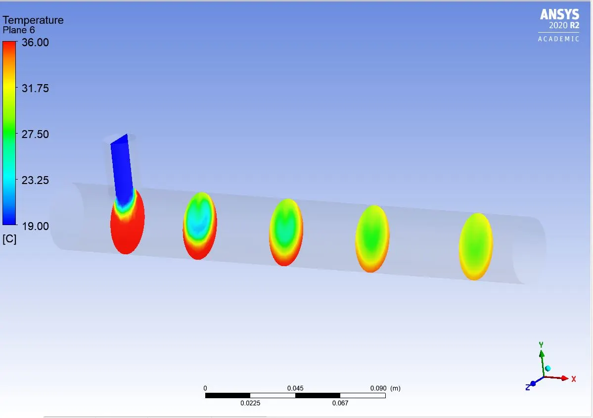
                                           Temperature contour plot across the plane for Tshort(Mr=2,K-epsilon method) 

                                              

                                                     

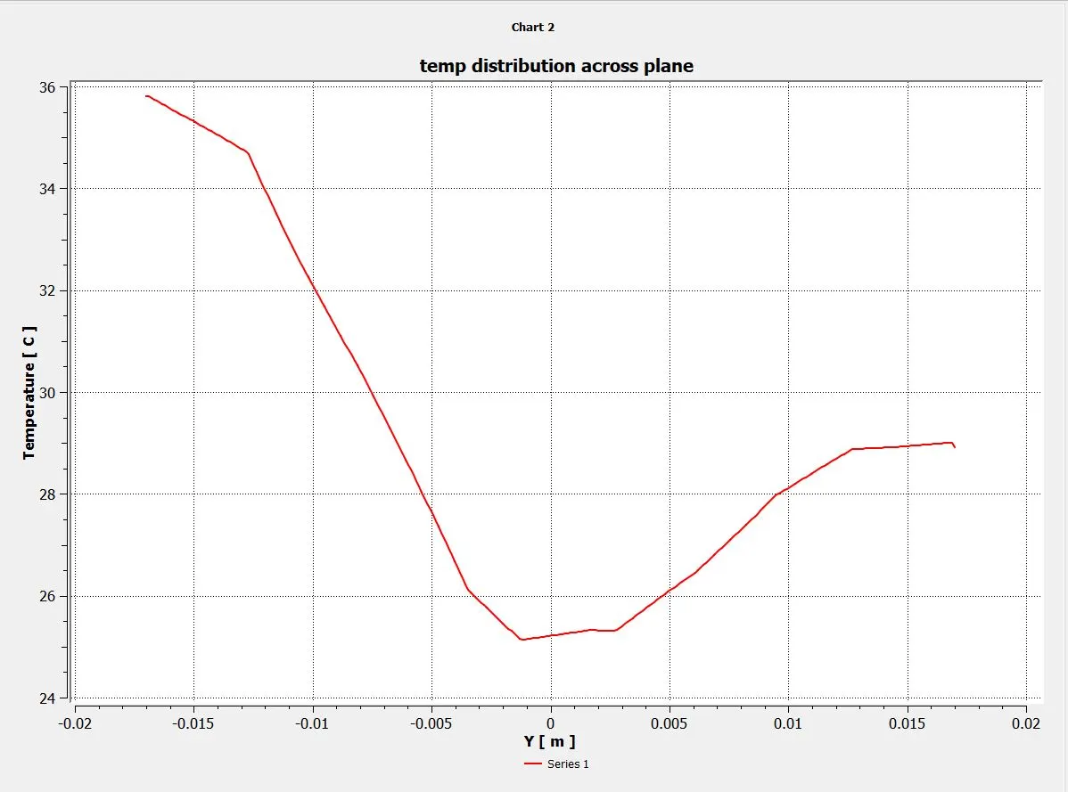
                                                Temperature line plot across the plane for Tshort(Mr=2,K-epsilon method) 

 As the cold fluid is entering from the top, the upper wall temperature is relatively cool as compared to the lower wall and as the mixing process going on it will reach a steady state and at the centre we can see a temperature of around 25˚C .

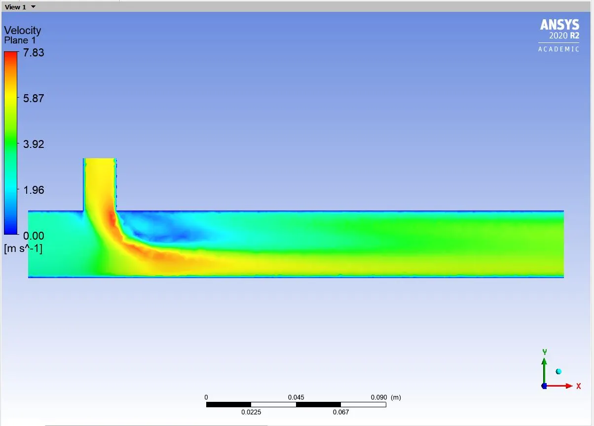
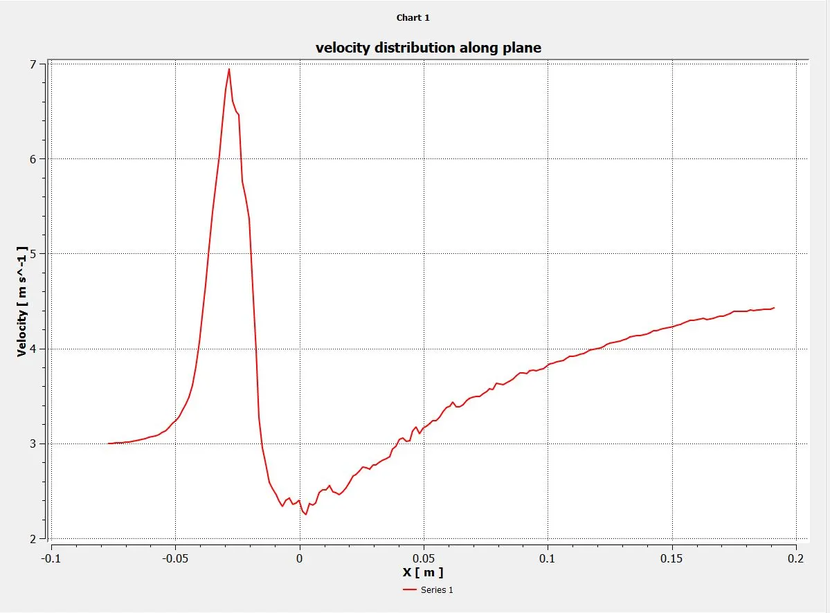
velocity along the plane:

                                               

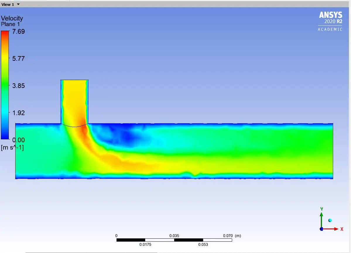
                                                        velocity contour plot along the plane for Tshort(Mr=2,K-epsilon method)

                                                       

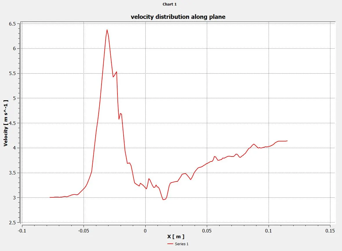
                                                         Velocity line plot along the plane for Tshort(Mr=2,K-epsilon method) 

It is clear from the plots that velocity reached a maximum value during mixing and and a value of 4.1m/s at the outlet.

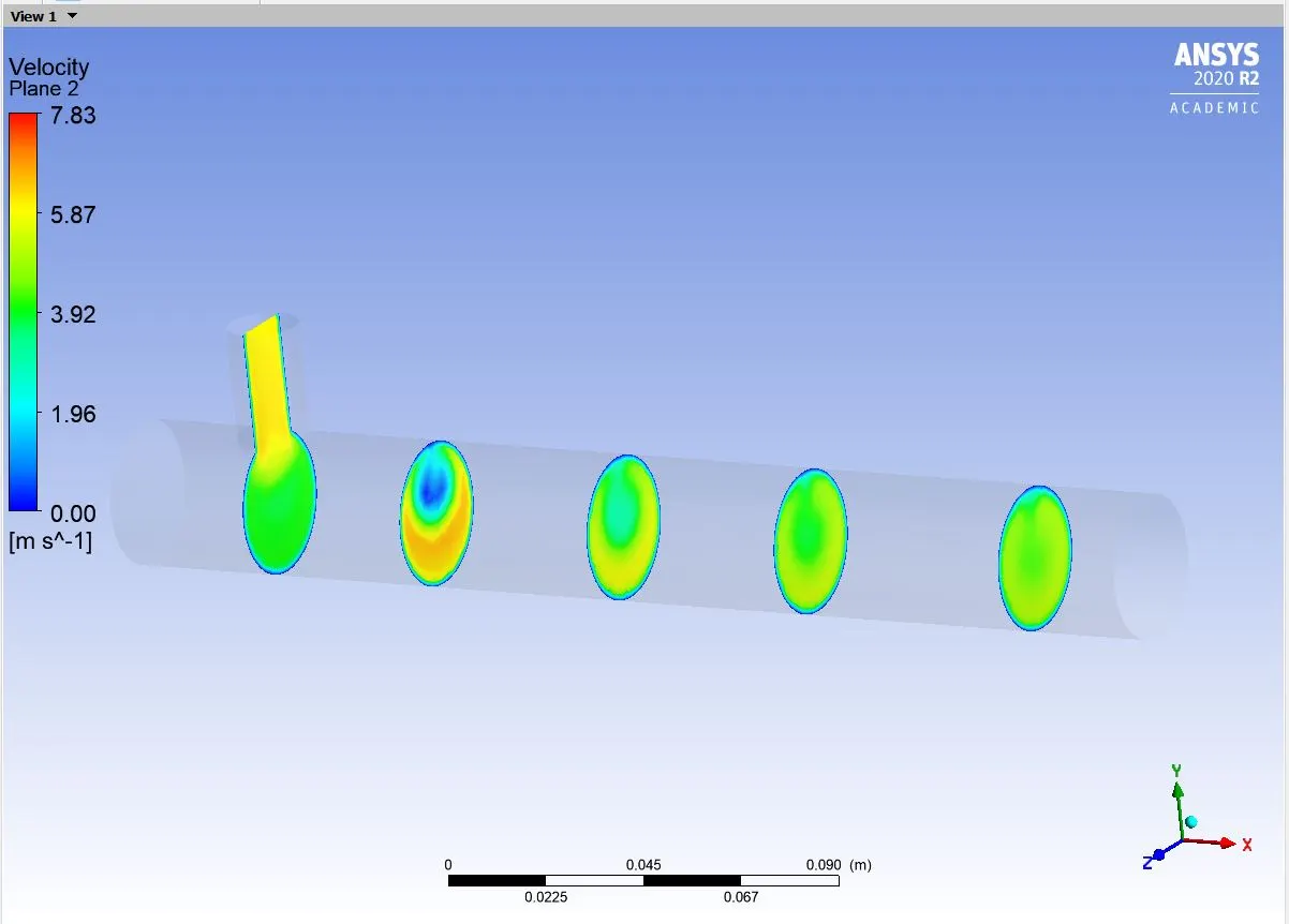
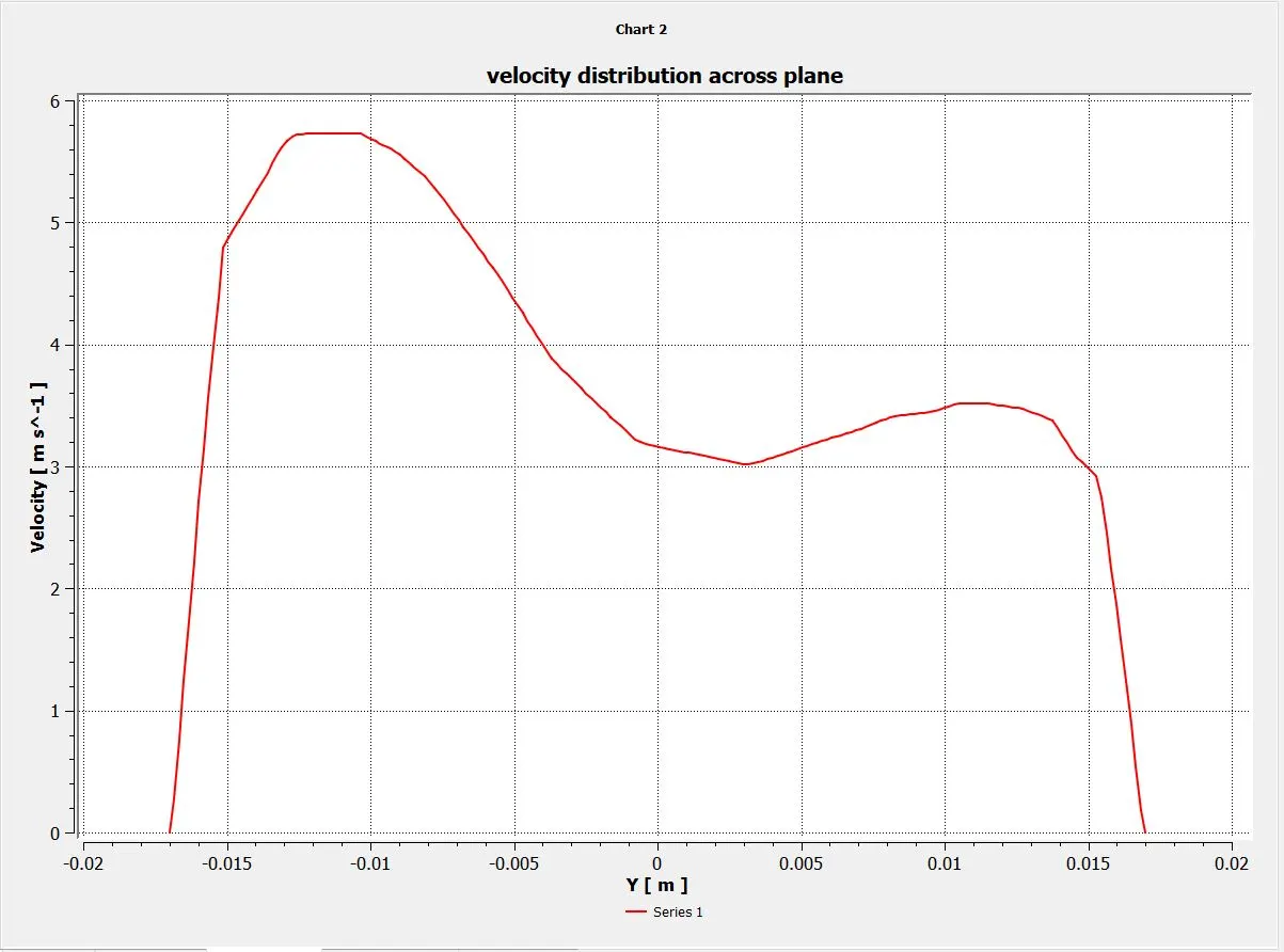
velocity across the plane:

                                                                         

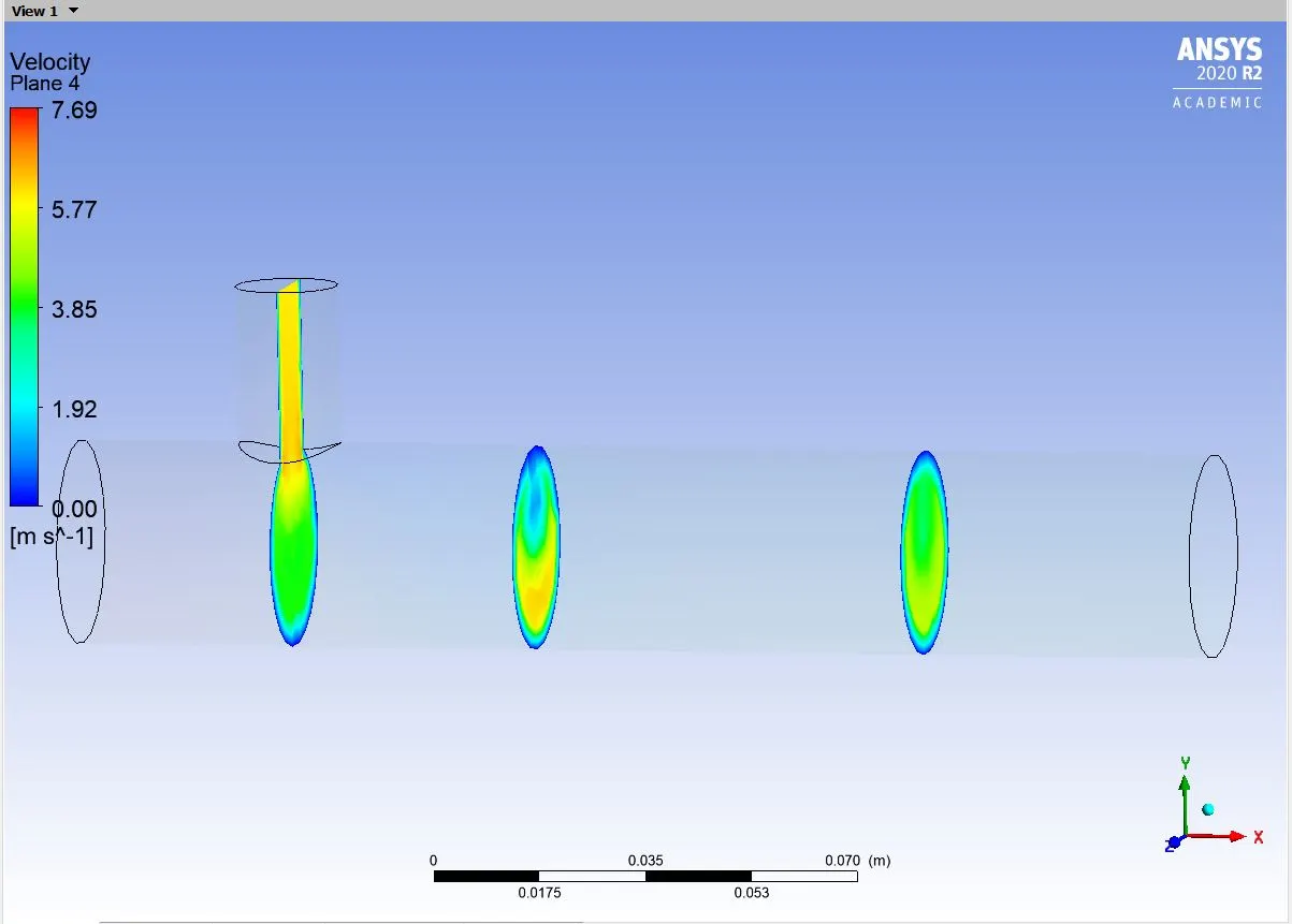
                                                                          velocity contour plot across the plane for Tshort(Mr=2,K-epsilon method)

                                                                       

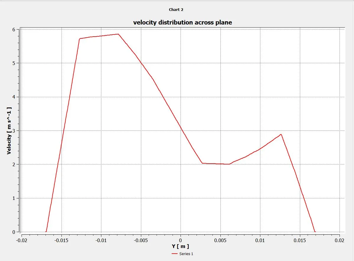
                                                                          velocity line plot across the plane for Tshort(Mr=2,K-epsilon method)

As we all know because of shear stress the velocity at the boundaries will be zero and velocity is maximum at a distance of 0.01mts downwards from the centre.

For momentum ratio=4, using k-epsilon residual method

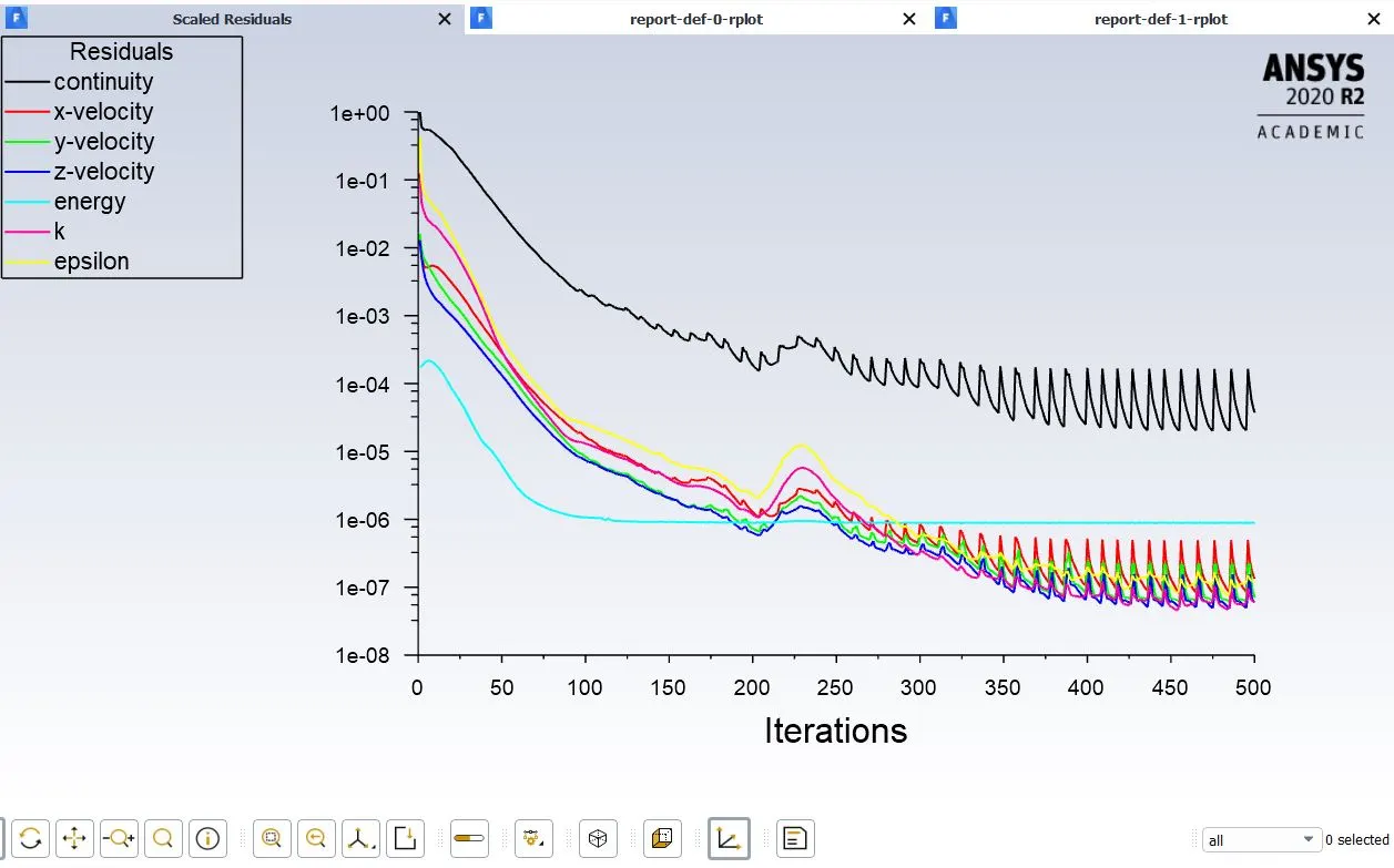
       Residual values for T-short mr=4 and k-epsilon

     

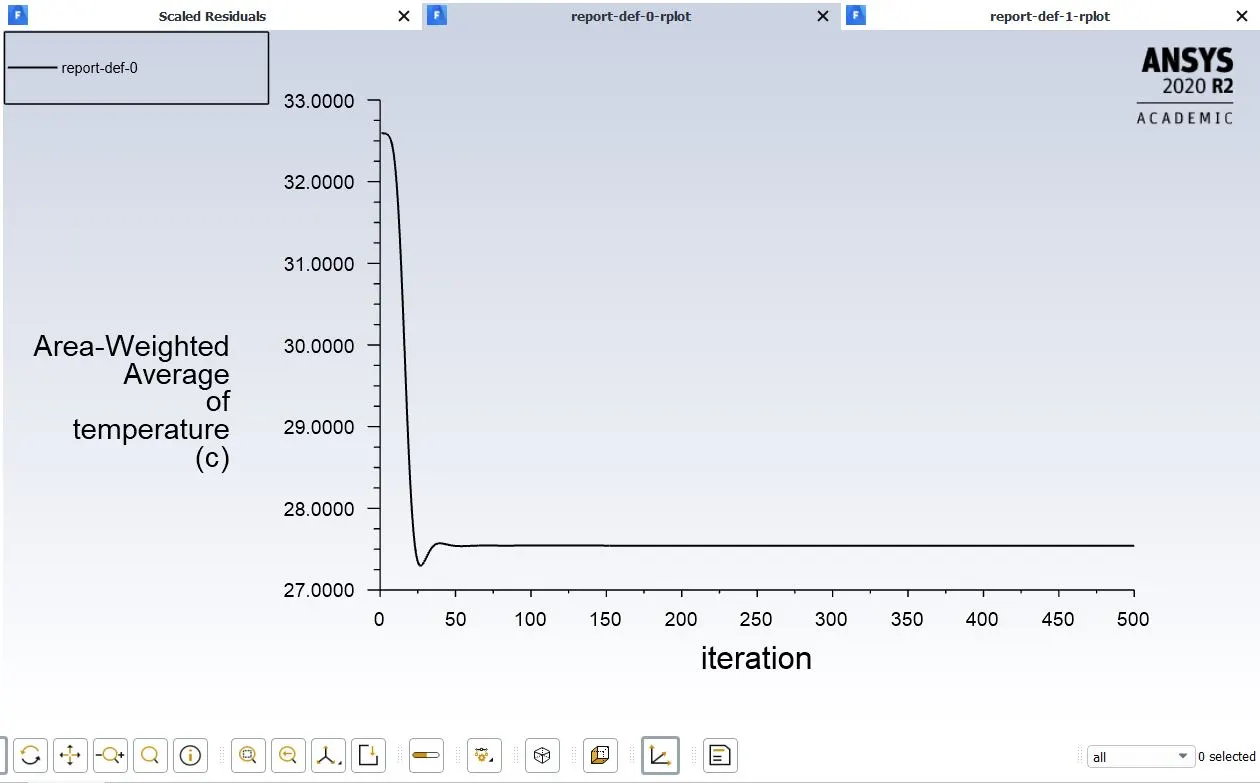
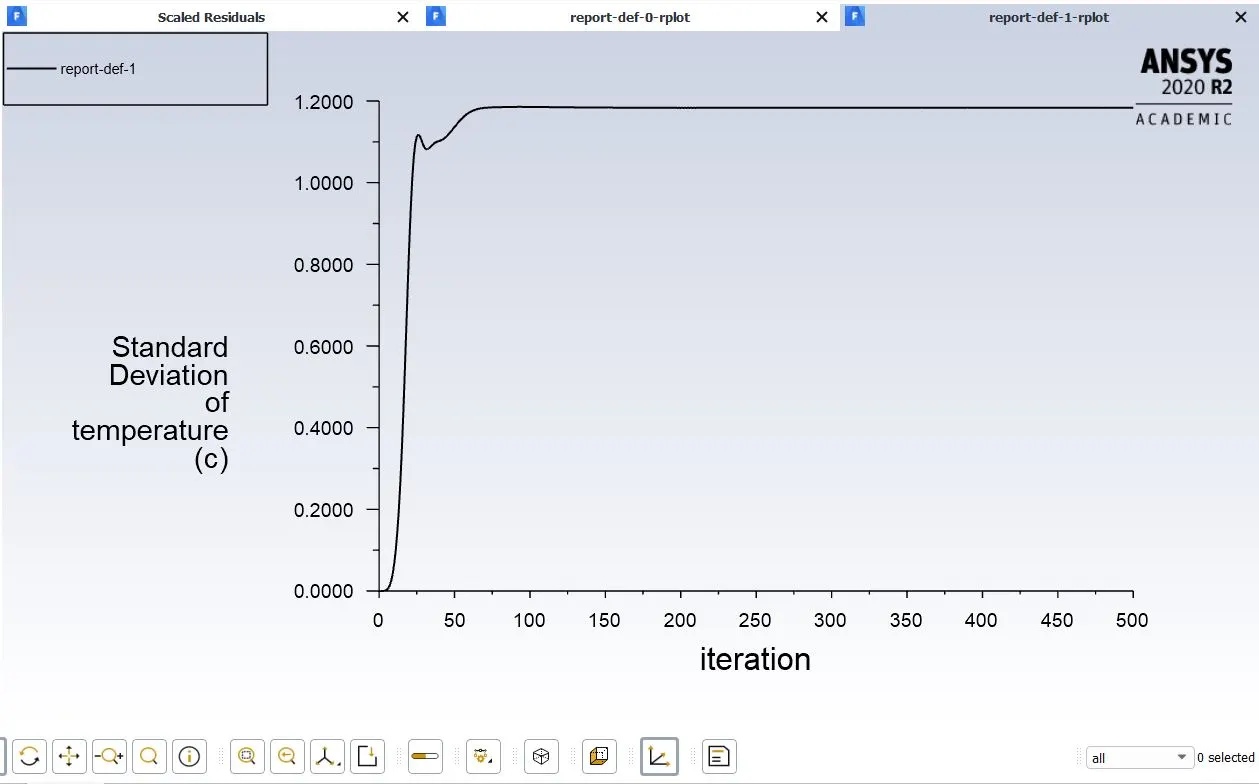
Area weighted average of temperature  for k-epsilon                                Standard deviation of temperature for k-epsilon

Results:

For momentum ratio=4, using k-epsilon residual method

Temperature along the plane:

                                                           

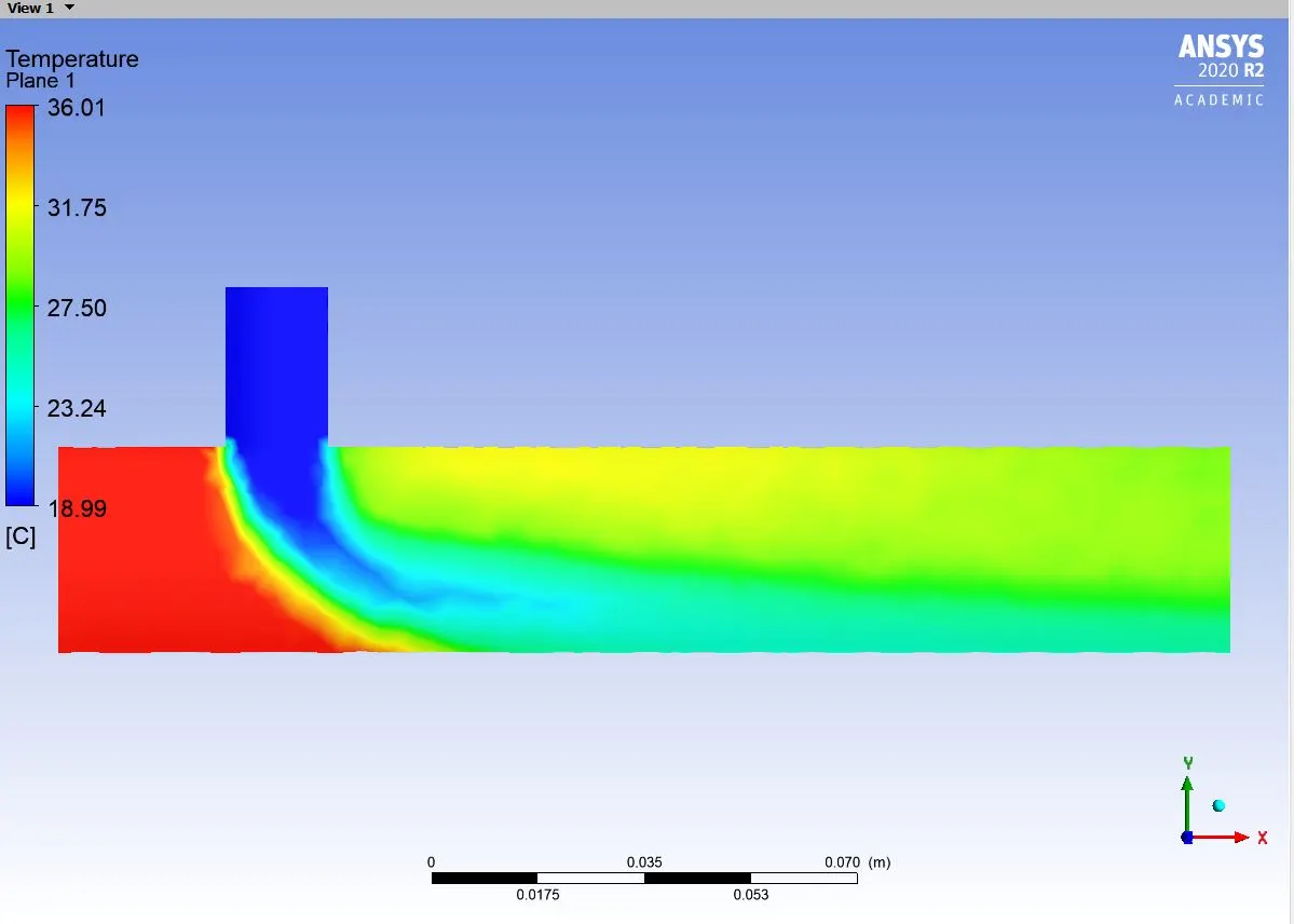
                                                            Temperature contour plot along the plane for Tshort(Mr=4,K-epsilon method) 

                                                         

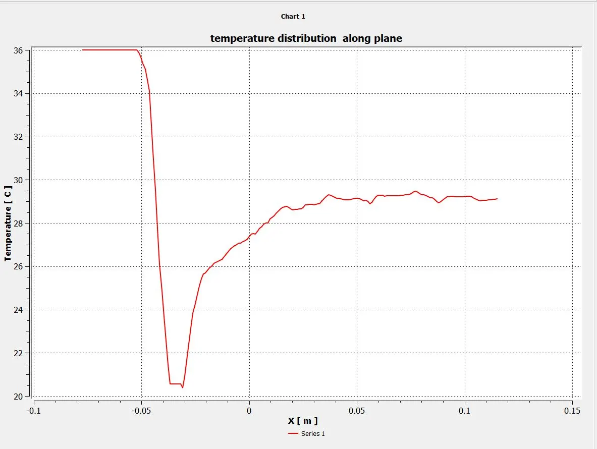
                                                       Temperature line plot along the plane for Tshort(Mr=4,K-epsilon method)

Temperature across the plane

:                                                      

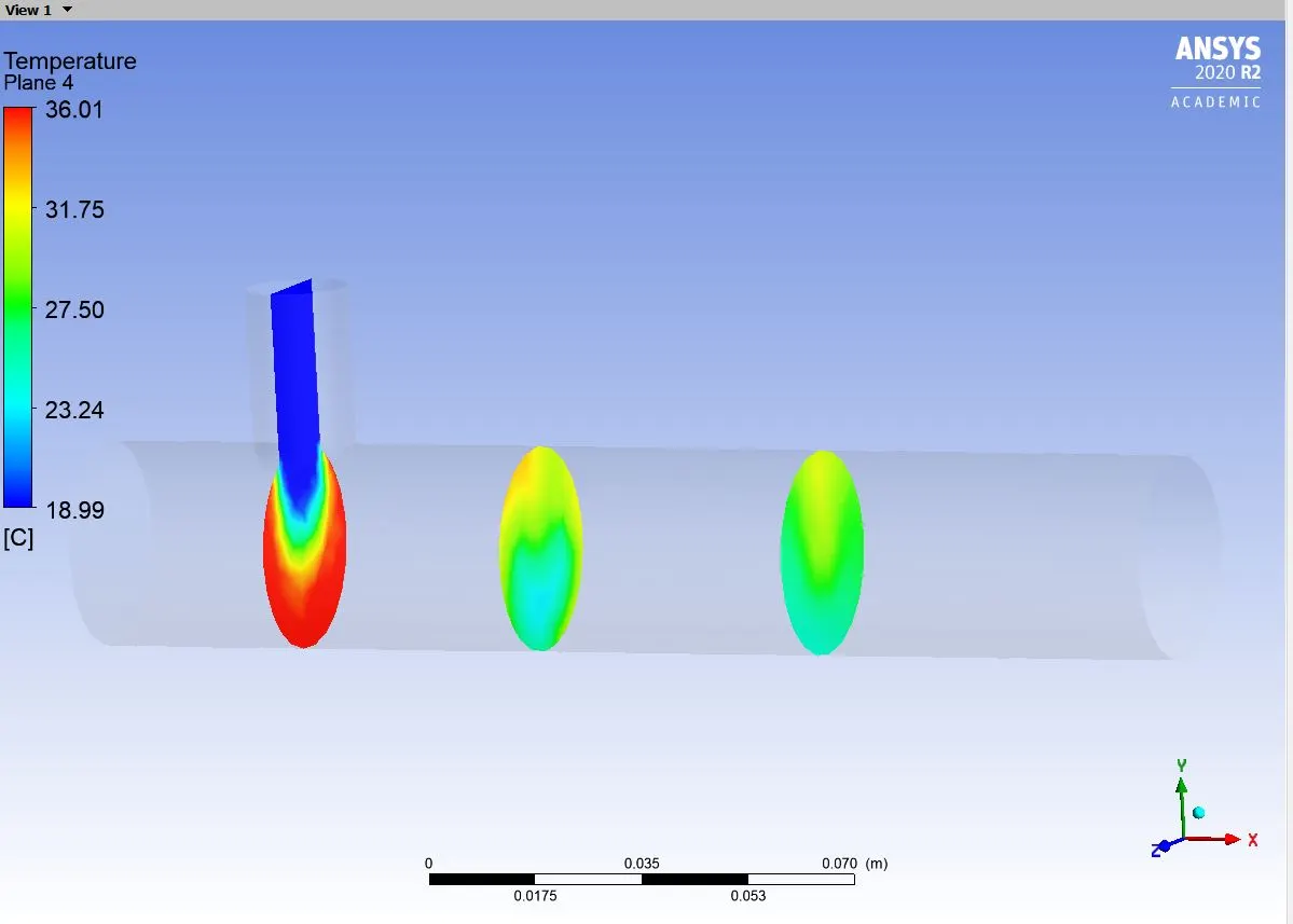
                                                    Temperature contour plot across the plane for Tshort(Mr=4,K-epsilon method) 

                                                                  

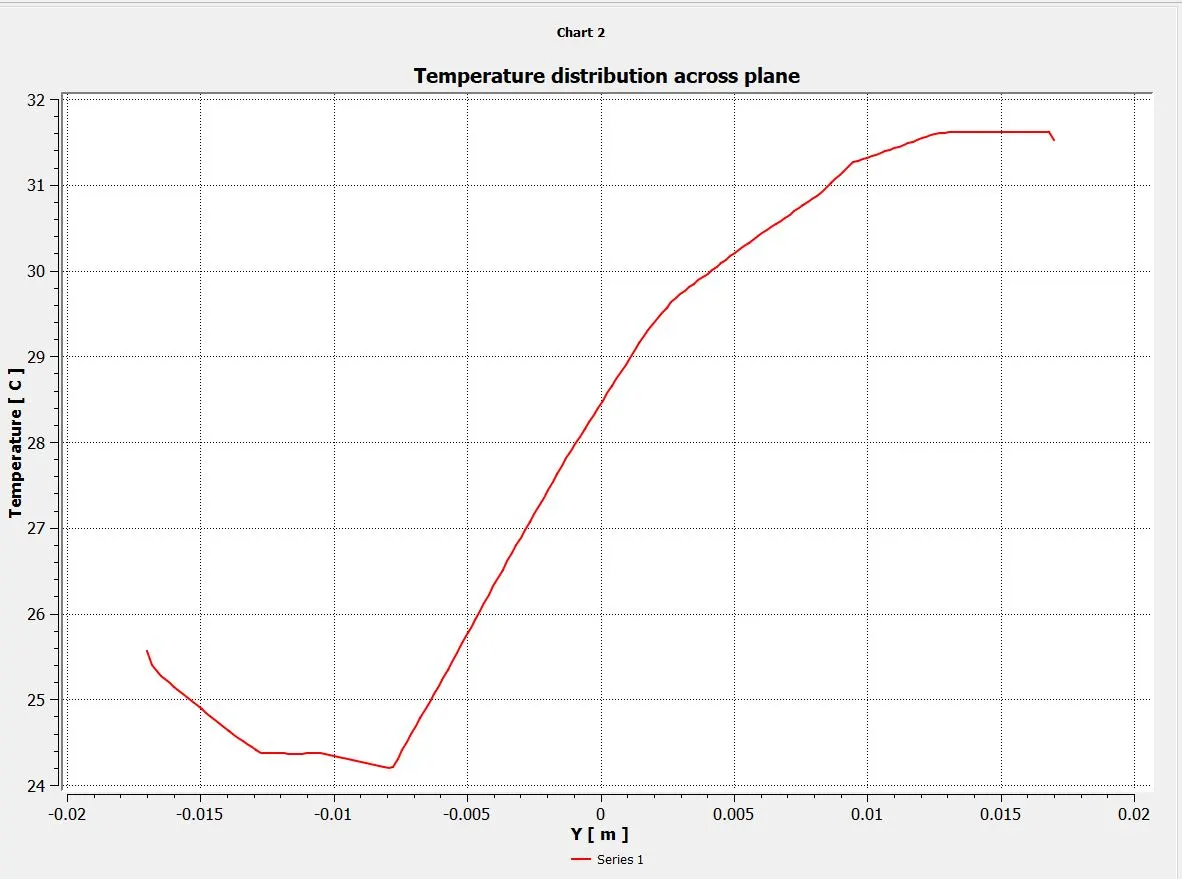
                                                             Temperature line plot across the plane for Tshort(Mr=4,K-epsilon method) 

velocity along the plane: 

                                                            

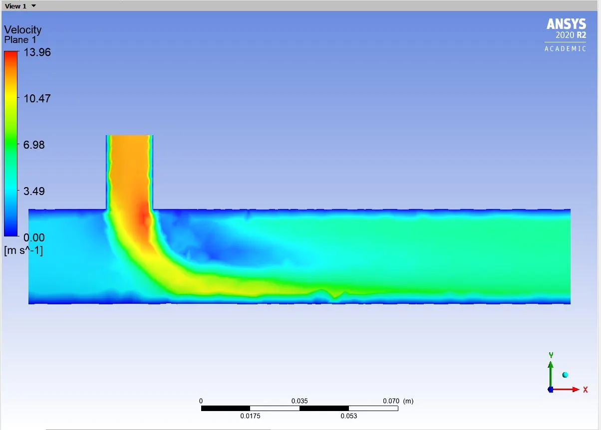
                                                               velocity contour plot along the plane for Tshort(Mr=4,K-epsilon method) 

                                                                                                          

                                                              

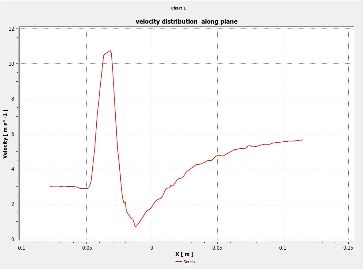
                                                               velocity line plot along the plane for Tshort(Mr=4,K-epsilon method)

 velocity across the plane:   

                                                            

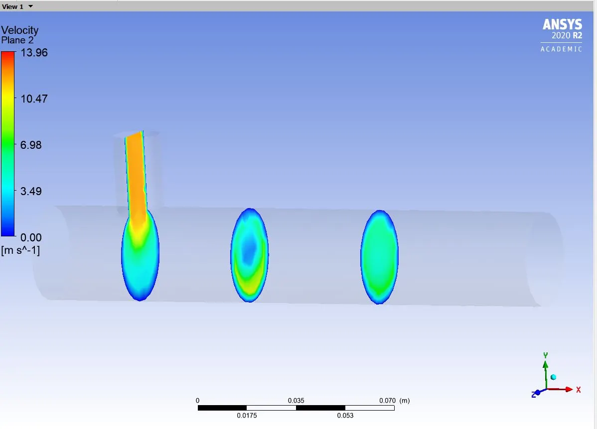
                                                                 velocity contour plot across the plane for Tshort(Mr=4,K-epsilon method) 

                                                                                                          

                                                        

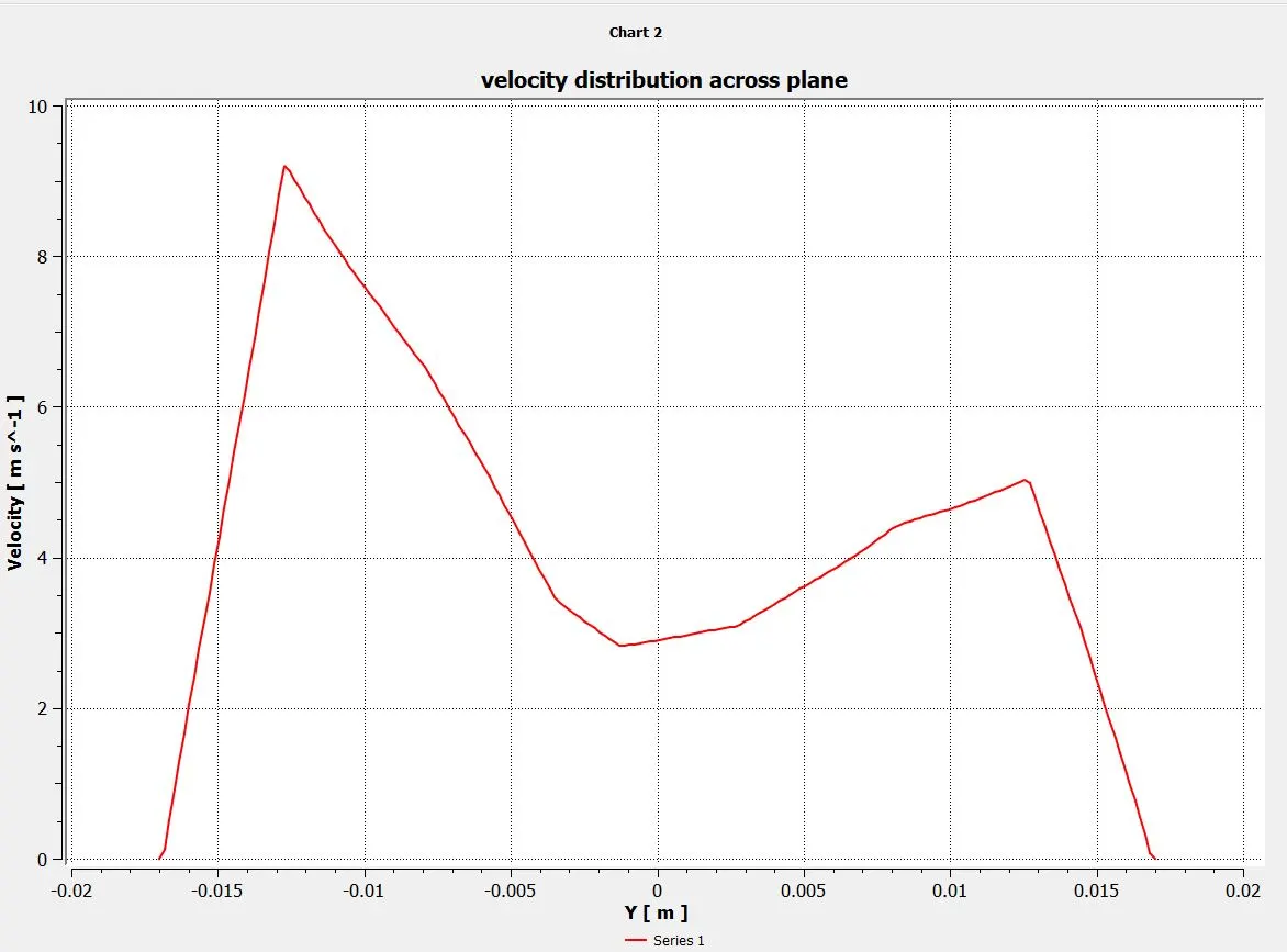
                                                             velocity line plot alcross the plane for Tshort(Mr=4,K-epsilon method) 

Case: 2 T- mixing in long tube  

Geometry:

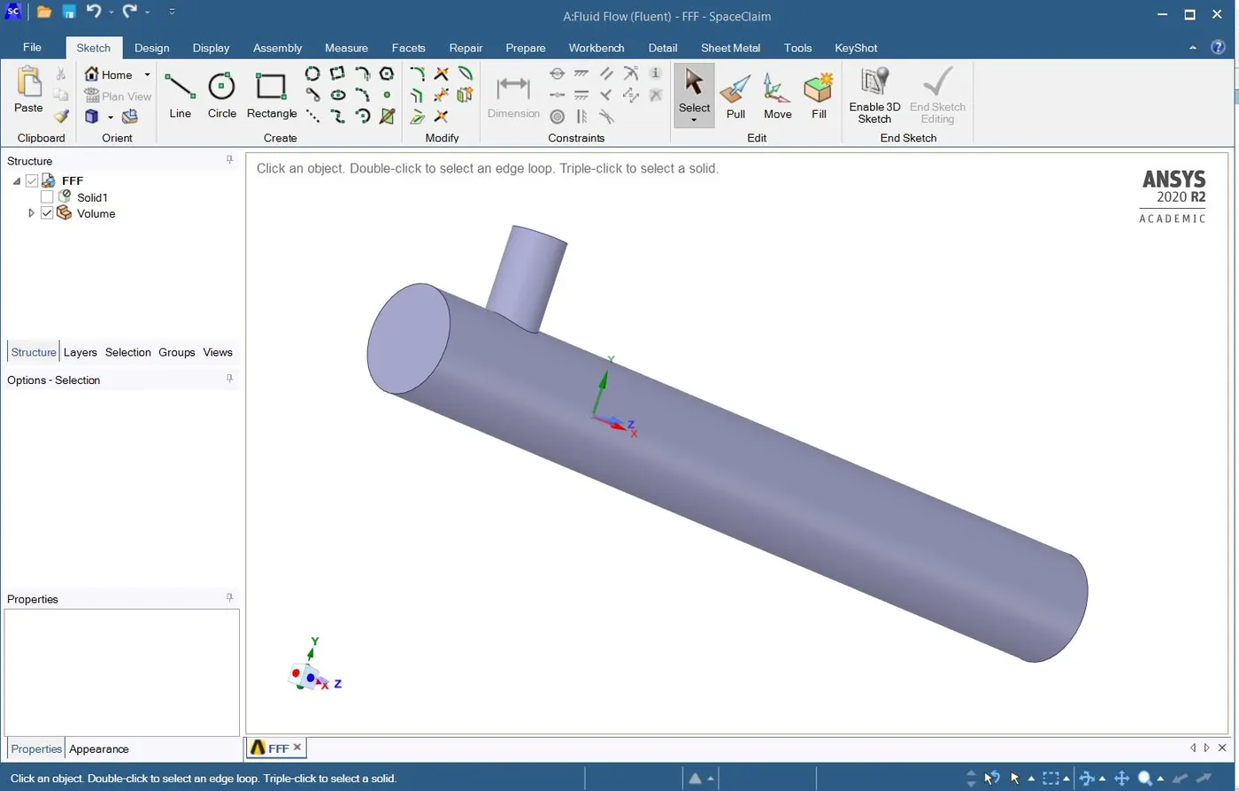
                                                                             space claim fluid volume   

 Meshing:

      

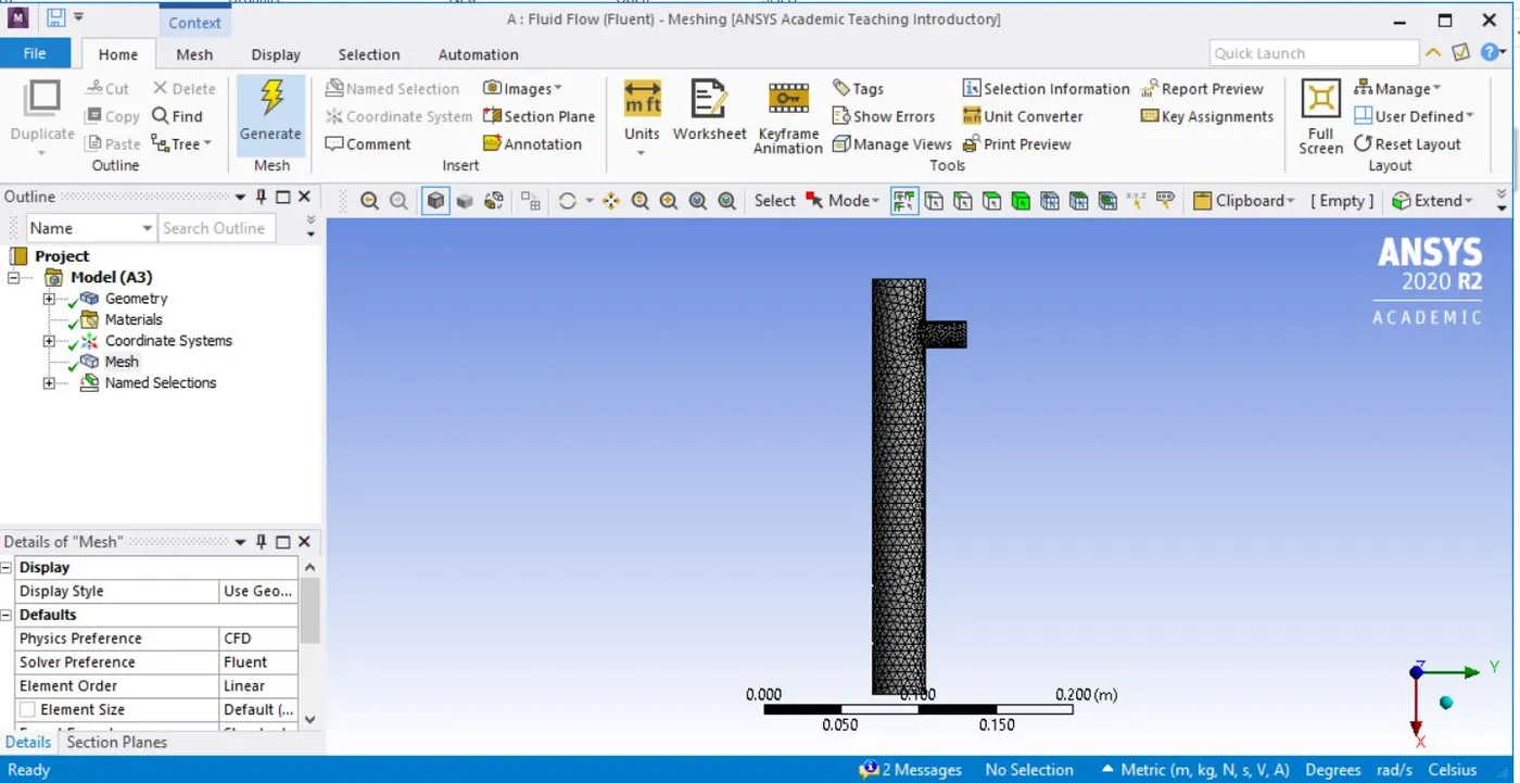
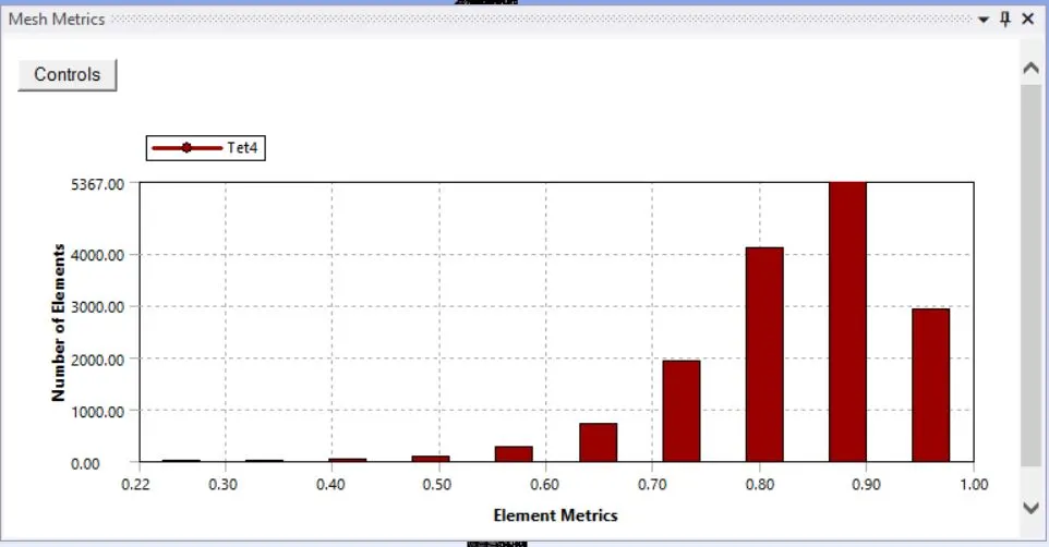
                                          Generated mesh                                                                                         Mesh quality                                                                      

 Setup:

For momentum ratio=2, using k-epsilon residual method

 

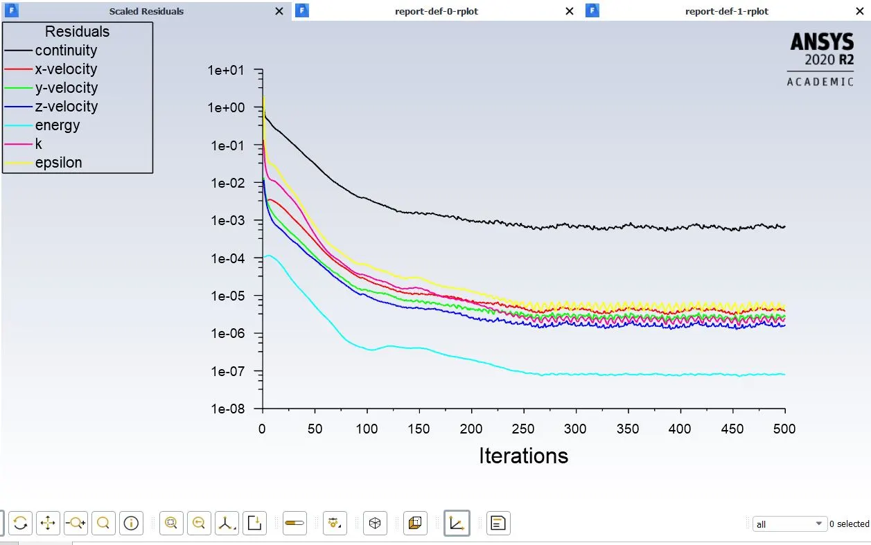
                                                              Residual values for T-long mr=2 and k-epsilon    

    

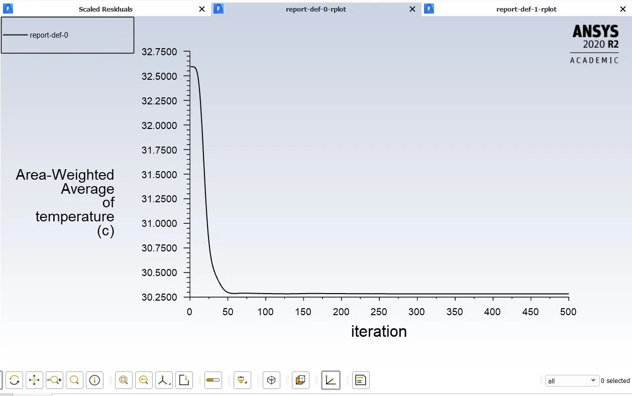
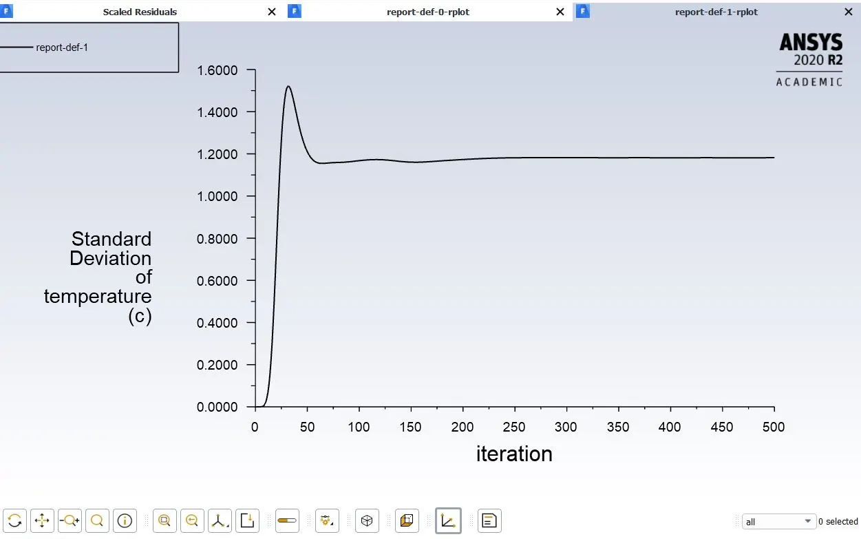
  Area weighted average of temperature  for k-epsilon                           Standard deviation of temperature for k-epsilon

Results:

For momentum ratio=4, using k-epsilon residual method

Temperature along the plane:

                                                                                               

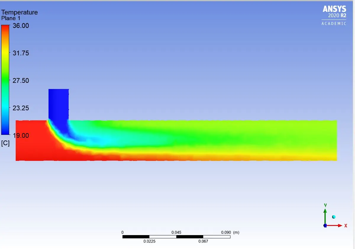
                                                                                    Temperature contour plot along the plane for Tlong(Mr=2,K-epsilon method) 

                                                                                                         

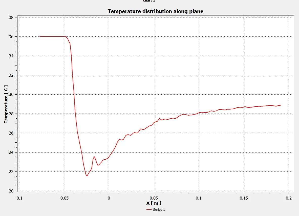
                                                                                                 Temperature line plot along the plane for Tlong(Mr=2,K-epsilon method) 

Temperature across the plane: 

                                                                                                     

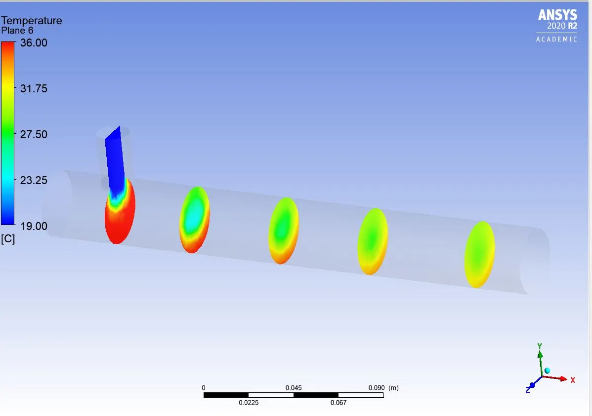
                                                                                                 Temperature contour plot across the plane for Tlong(Mr=2,K-epsilon method)

                                                                                                        

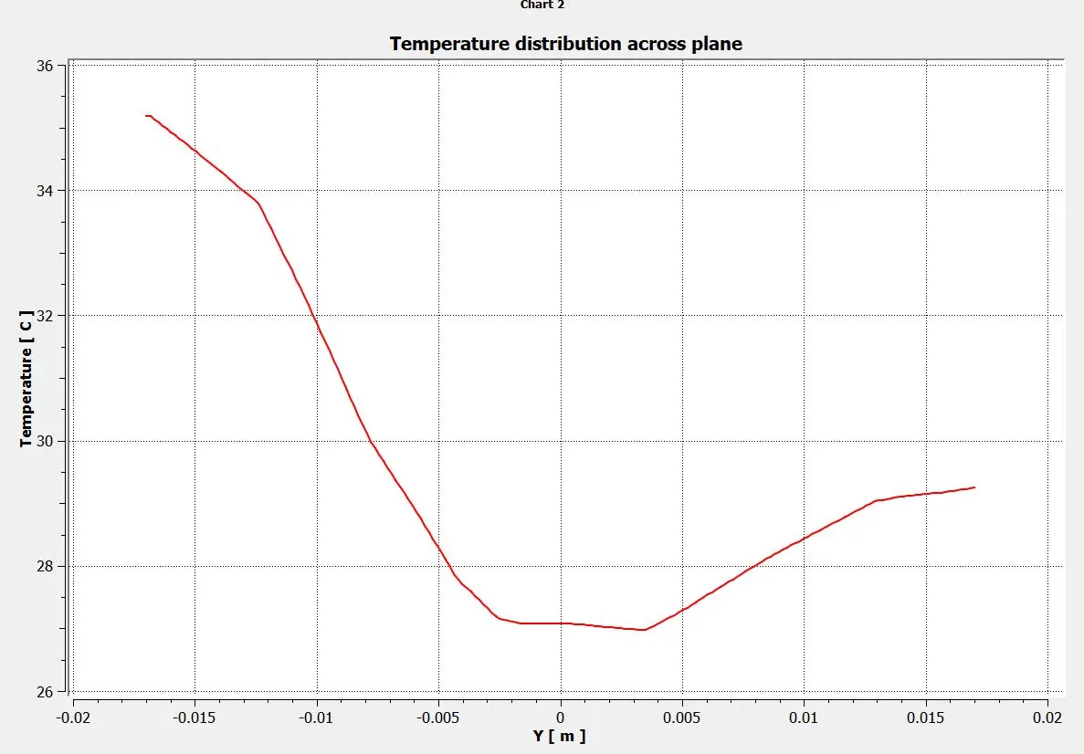
                                                                                                  Temperature line plot along the plane for Tlong(Mr=2,K-epsilon method) 

velocity along the plane:  

                                                                                               

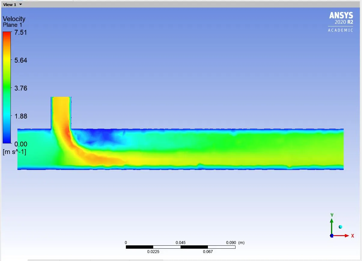
                                                                                               velocity contour plot along the plane for Tlong(Mr=2,K-epsilon method) 

                                                                                                 

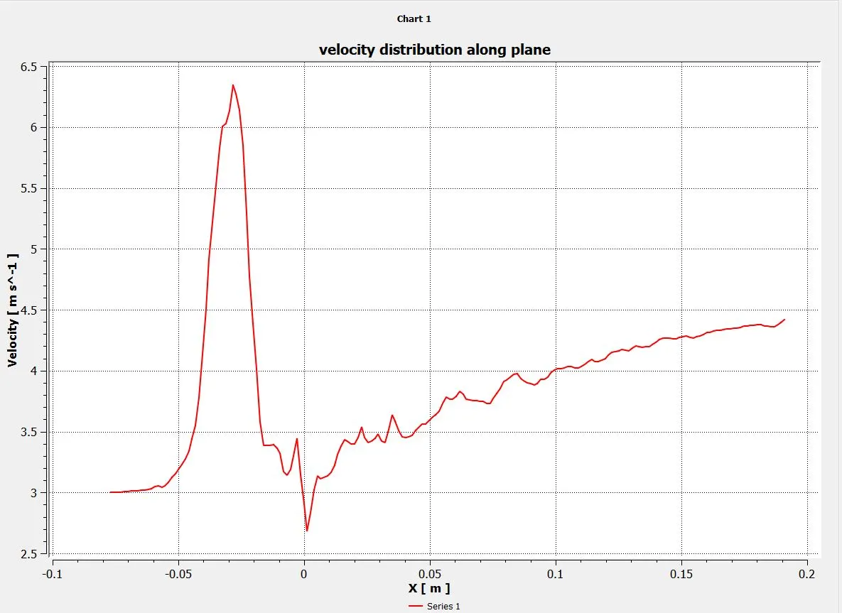
                                                                                                     velocity line plot along the plane for Tlong(Mr=2,K-epsilon method) 

velocity across the plane: 

                                                                                       

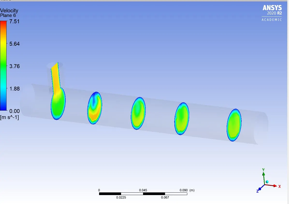
                                                                                          Velocity contour plot across the plane for Tlong(Mr=2,K-epsilon method)

                                                                                     

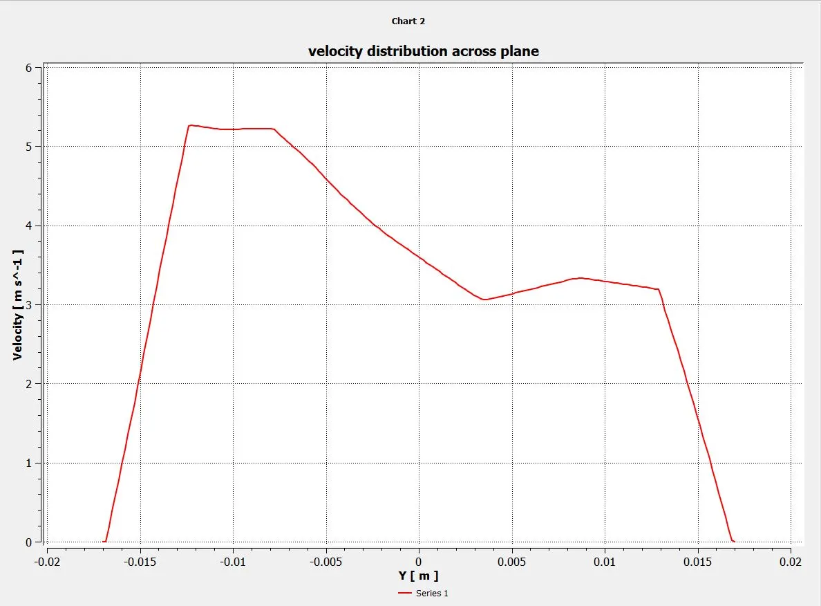
                                                                                                Velocity line plot across the plane for Tlong(Mr=2,K-epsilon method) 

For momentum ratio=4, using k-epsilon residual method

        

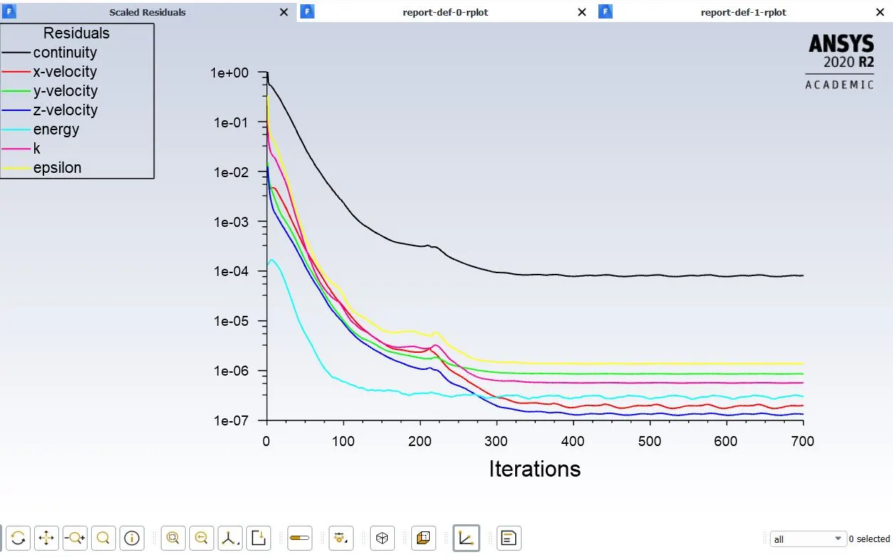
                  Residual values for T-long mr=4 and k-epsilon

   

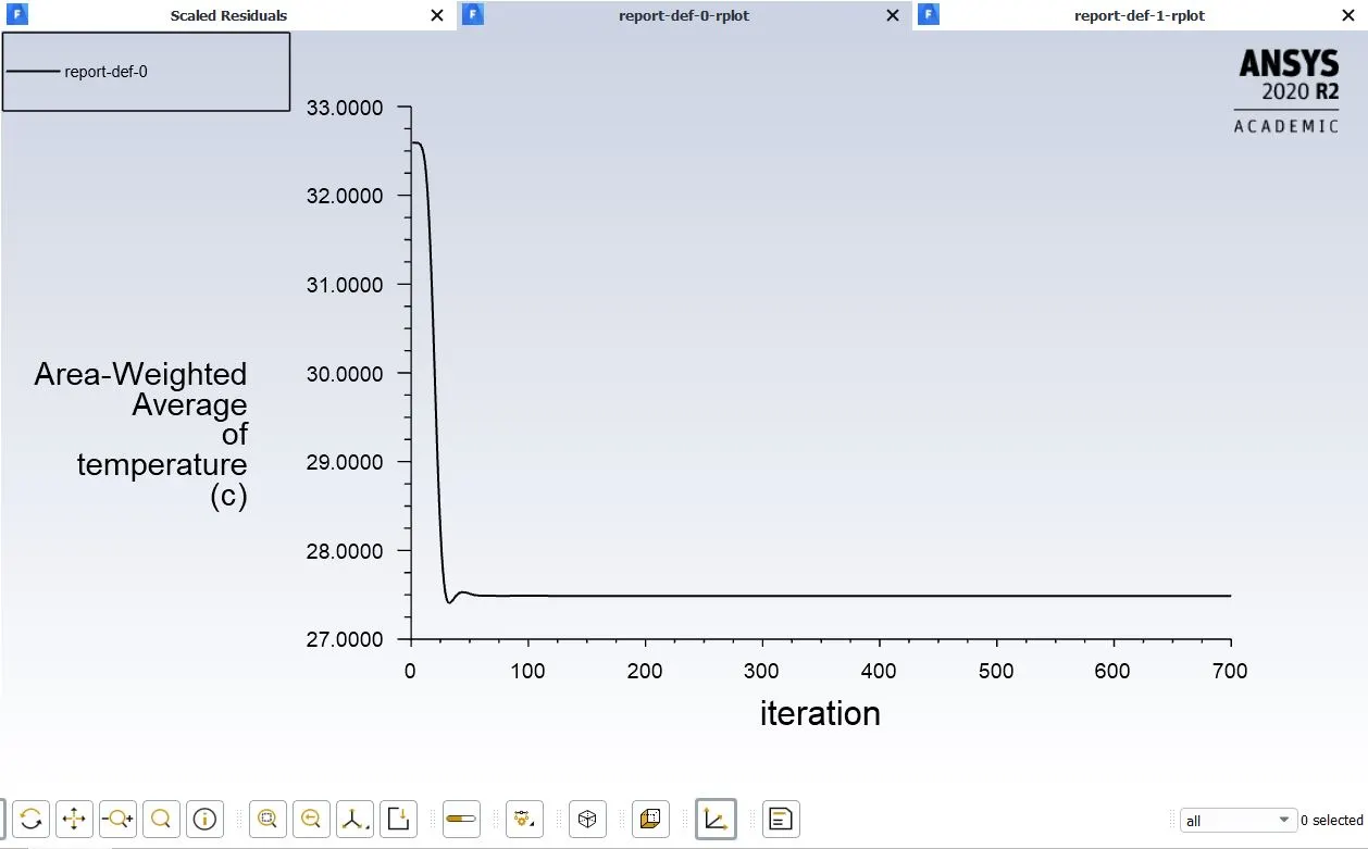
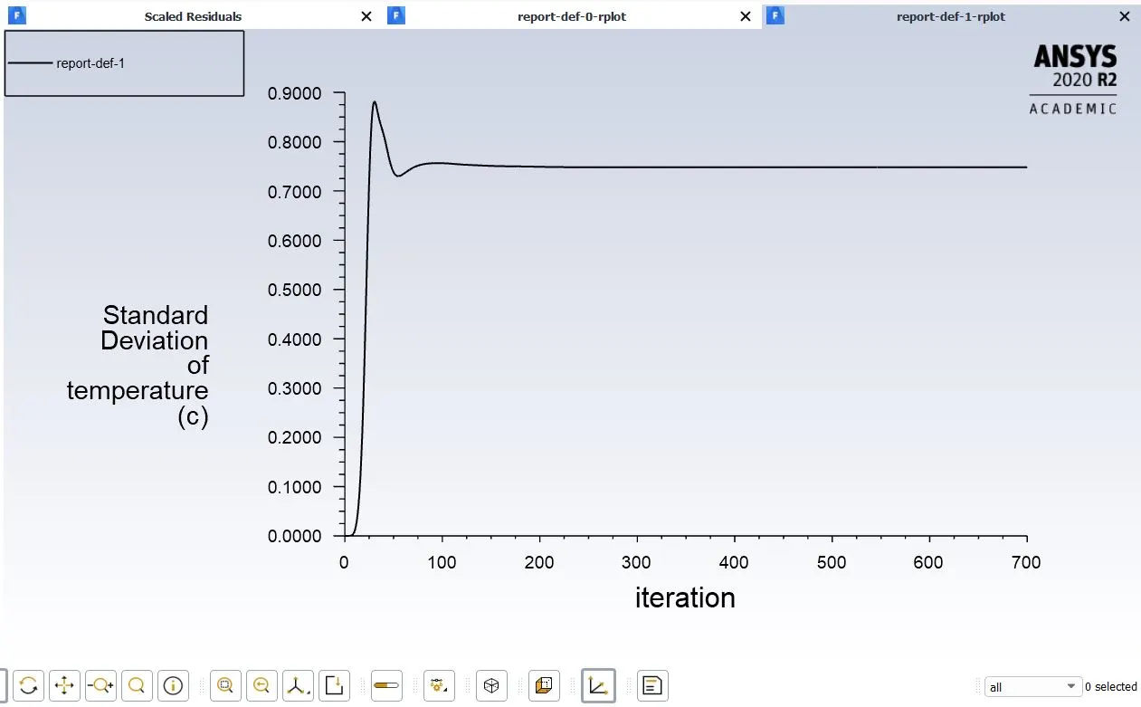
         Area weighted average of temperature  for k-epsilon                          Standard deviation of temperature for k-epsilon                                                                                                                                                                                                                       

Results:

For momentum ratio=4, using k-epsilon residual method

Temperature along the plane:     

                                                            

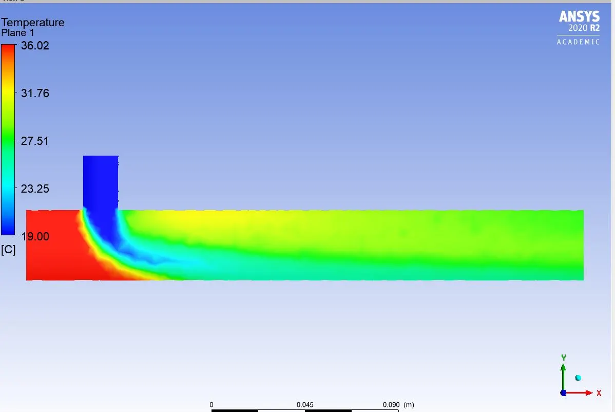
                                                                Temperature contour plot along the plane for Tlong(Mr=4,K-epsilon method) 

                                                                       

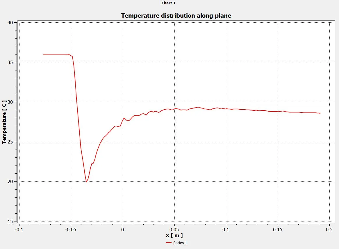
                                                                          Temperature line plot along the plane for Tlong(Mr=4,K-epsilon method) 

Temperature across the plane: 

                                                                

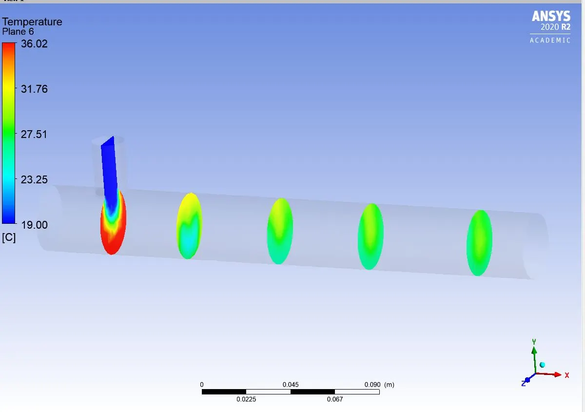
                                                                    Temperature contour plot across the plane for Tlong(Mr=4,K-epsilon method) 

                                                                  

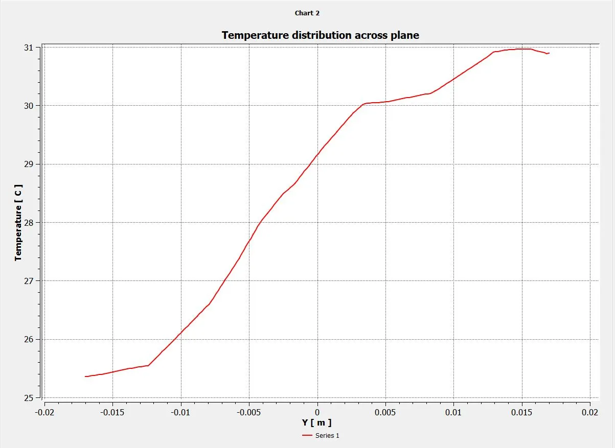
                                                                      Temperature line plot across the plane for Tlong(Mr=4,K-epsilon method) 

 velocity along the plane:

                                                            

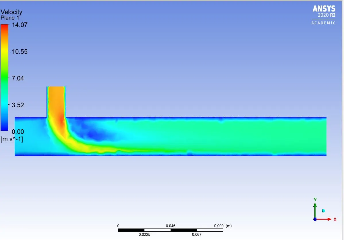
                                                                Velocity contour plot along the plane for Tlong(Mr=4,K-epsilon method) 

                                                                     

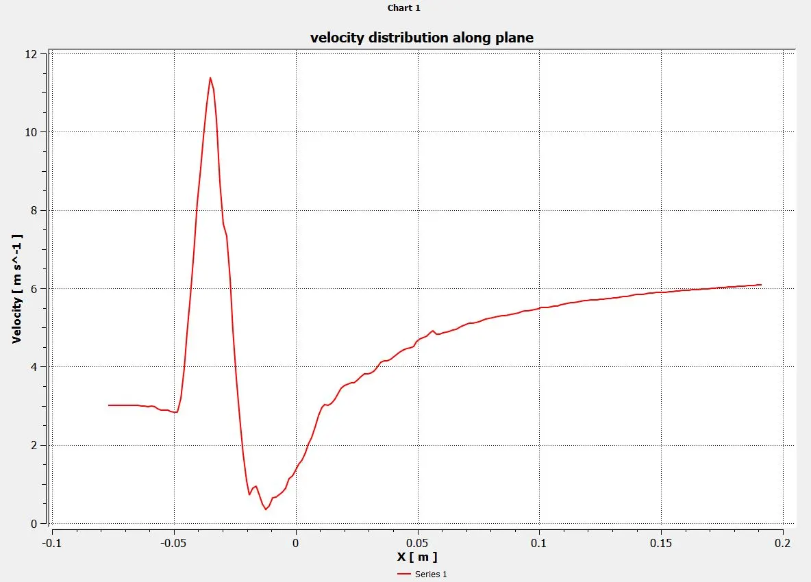
                                                                            Velocity line plot along the plane for Tlong(Mr=4,K-epsilon method) 

velocity across the plane: 

                                                                           

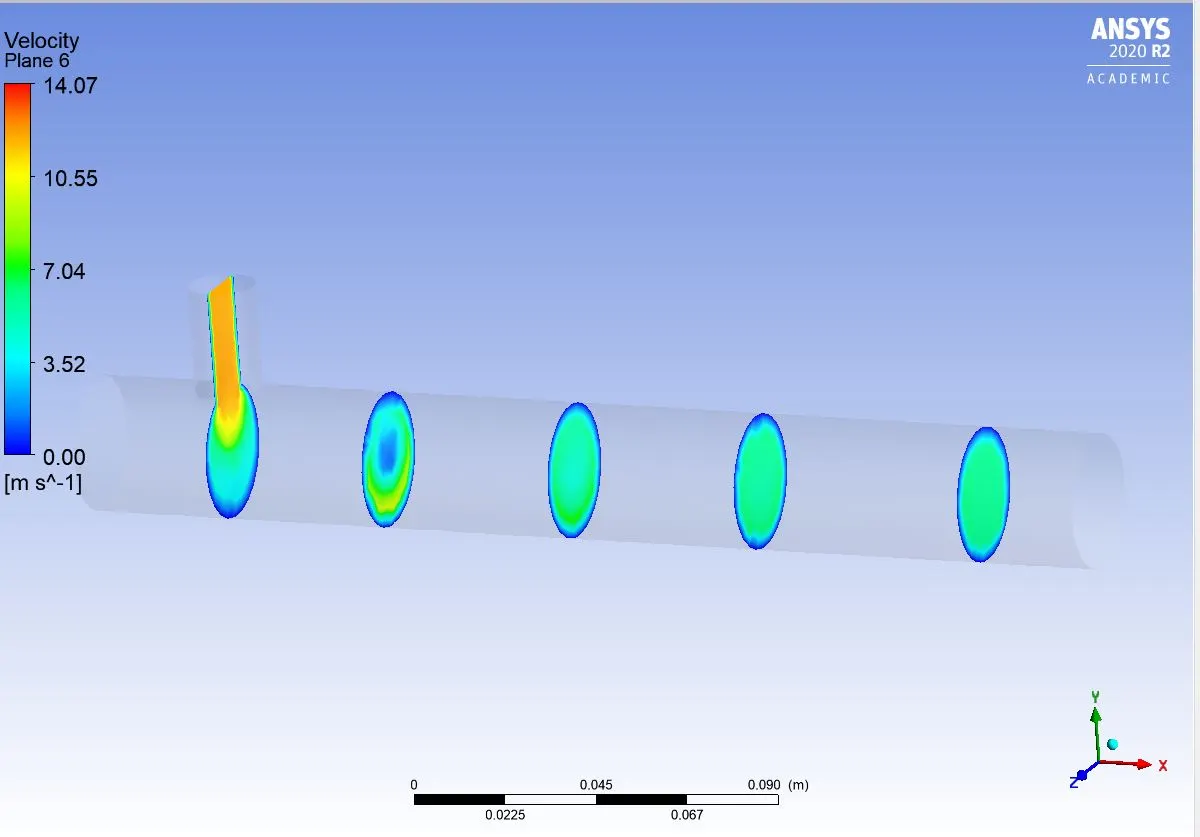
                                                                         Velocity contour plot across the plane for Tlong(Mr=4,K-epsilon method) 

                                                                             

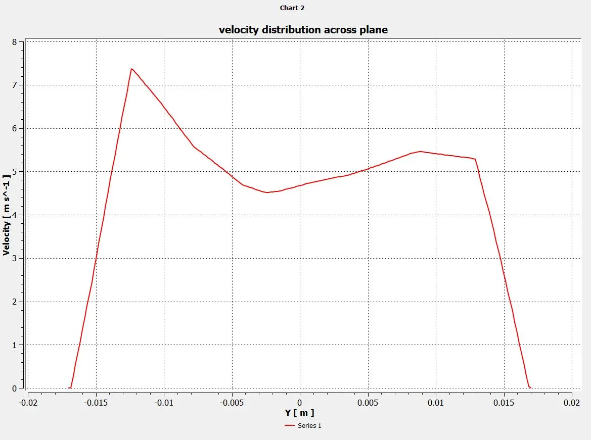
                                                                               Velocity contour plot across the plane for Tlong(Mr=4,K-epsilon method) 

Mesh independent study for T-long mixing using momentum ratio=2

L.H.S: Default meshing

R.H.S: Refined meshing

Meshing:

         

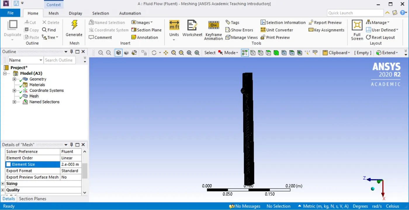
Element size: 0.013853(default)                                                                              Element size: 0.002                                                

Nodes: 3432                                                                                                                 Nodes: 28282                   

Elements: 15368                                                                                                          Elements: 140025                                                                             

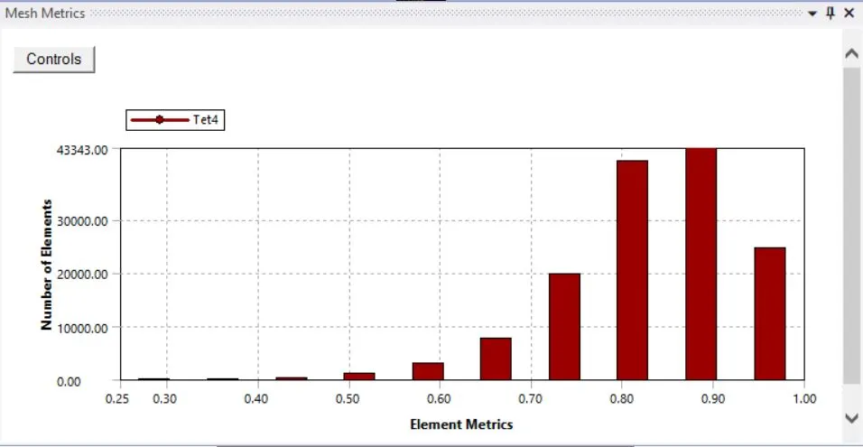
Mesh Quality:

             

Residuals:

                 

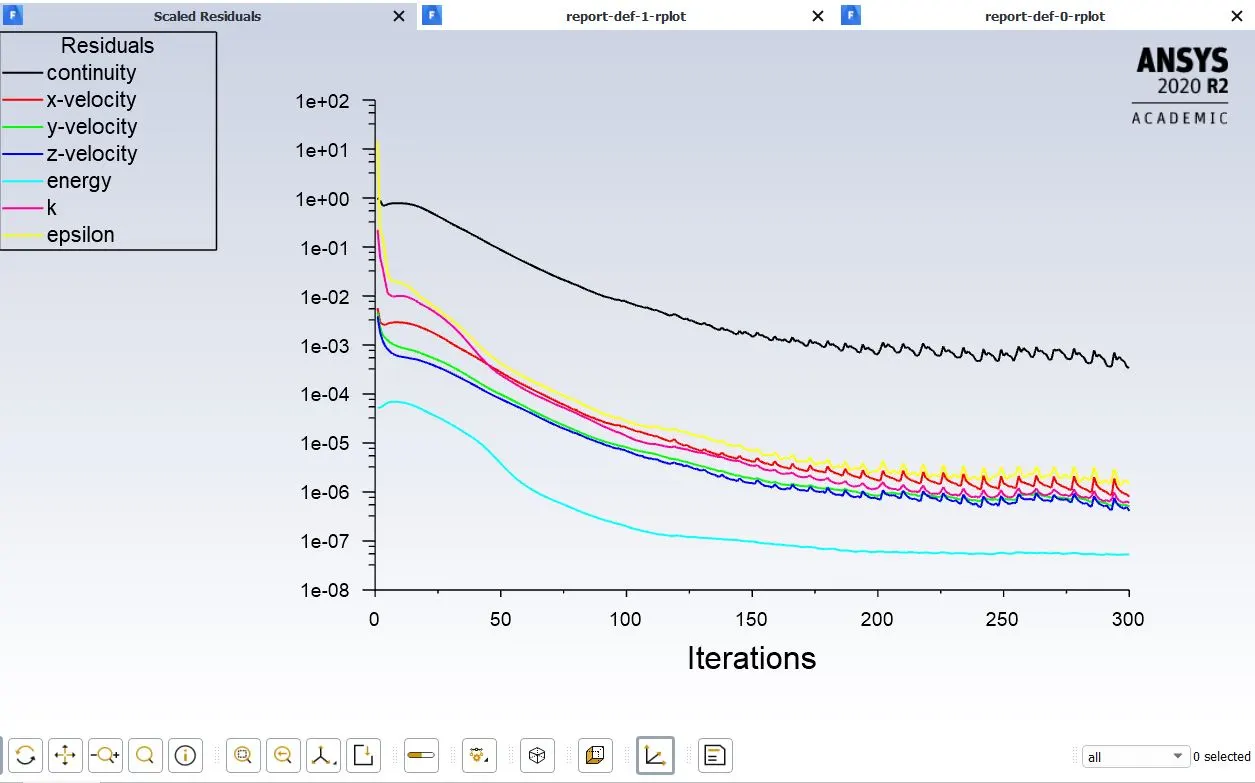
solution converged at 250 iterations                                                                                        solution converged at 200 iterations       

Area weighted average of Temperature:

                    

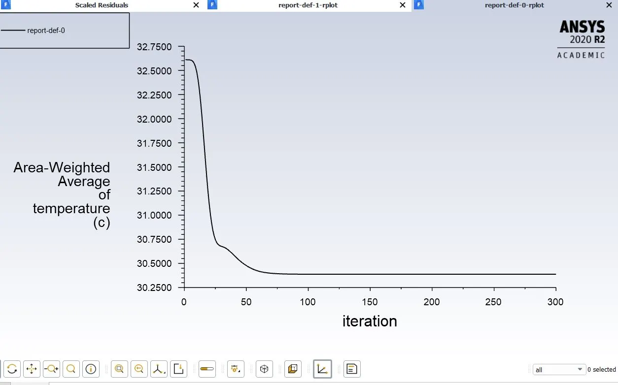
Standard deviation:

       

Comparison of Results:

Temperature along the plane:

           

              

Temperature across plane:

             

Velocity along the plane:

               

               

Velocity across plane:

             

                    

 Comparison of Results:

	T-Short		T-Long
	Momentum ratio =2	Momentum ratio =4	Momentum ratio =2	Momentum ratio =4
Cell count	12583	12583	15368(default) 140025(refined)	15368(default) 140025(refined)
Average outlet temperature	30.25C	27.5C	30.25C	27.5C
Number of iterations for convergence	150(for k epsilon) 350(for k-omega)	350	250	325

 Conclusions:

• Change of length does not change have much effect on the outlet temperature 
• Change of momentum ratio have a great effect by reducing the temperature of 3˚C, this is because of increase in velocity increases turbulence during mixing.
• Coming to the turbulence model k-epsilon gives less standard deviation than k-omega, but during analysis of T-short with momentum ratio=2, k-epsilon does not give conversed solution even after 1000 iterations.
• Decrease in mesh size gives good velocity and temperature distribution but it will take more time for iterations also it will affect in mesh quality.